
Join 1,000s of professionals who are building real-world skills for better forecasts with Microsoft Excel.
Issue #52 - Forecasting with ARIMA Part 7:
Improving Your Model
This Week’s Tutorial
Last week's tutorial taught you how to craft your first ARIMA model and tune it for the Sales dataset in the workbook. If you're new to this tutorial series, you can get all the previous tutorials here - just scroll down to the bottom of the page.
In this tutorial, you will investigate how to improve the first iteration of your ARIMA model by enriching the dataset to capture seasonality. As with all predictive modeling tasks, there's no guarantee this enrichment (also called feature engineering) will work.
However, you won't know until you try.
If you would like to follow along with today's tutorial (highly recommended), you will need to download the SalesTimeSeries.xlsx file from the newsletter's GitHub repository.
The Workbook So Far
I'm going to assume you've set up your workbook as described in Part 6 of this tutorial series. The following screenshot illustrates how your Python Code worksheet should be set up:
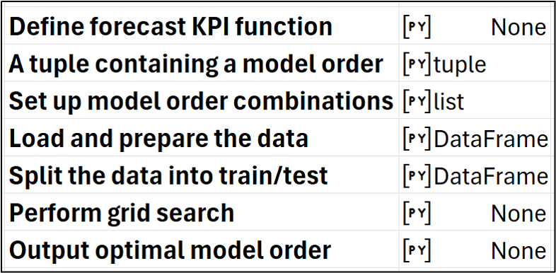
You will learn how to tweak the above to incorporate seasonality into the dataset to train the ARIMA model. The first step is to insert a new row into the Python Code worksheet:
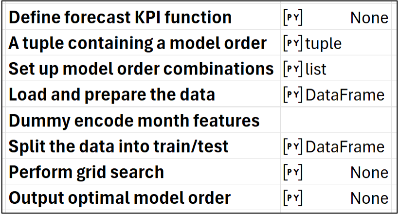
The added step will create exogenous features representing the month of the year.
Endogenous vs Exogenous Features
As discussed in Part 3 of this tutorial series, when it comes to using data to build better forecasts, the features you use fall into one of two categories. While there are technical definitions for the following, for this tutorial series, I will take an intuitive approach:
Endogenous means the feature comes from "inside" the time series target values. For example, a moving average calculated from the time series target values is endogenous.
Exogenous means the features come from "outside" the time series target values. For example, monthly marketing spend is an exogenous feature when monthly sales are the targets.
For the Sales dataset, we need to include exogenous features representing the month of the year so the ARIMA model can learn about seasonality.
However, ARIMA initially did not support exogenous features. Luckily, the statsmodels Python library provides an ARIMA model that can incorporate exogenous features.
So, you can add the months of the year to the Sales dataset, but how do you do that exactly?
Dummy Encoding
For brevity, I won't repeat everything from Part 3 of this tutorial series. Feel free to check it out if you're new to this series or if you need a refresher.
The goal of this tutorial is to build a better ARIMA forecasting model by providing the model with data in a form that allows it to learn about seasonality. While there are several techniques you can use for this, the easiest is to use dummy encoding.
Dummy encoding is a common technique in predictive modeling. So, not surprisingly, Python provides multiple ways to perform it.
In this tutorial, I'm going to use the pandas library's get_dummies() function. Another option would be to use the OneHotEncoder class from the scikit-learn library.
Here's the Python formula for creating a DataFrame of month names (i.e., a DataFrame of exogenous features):
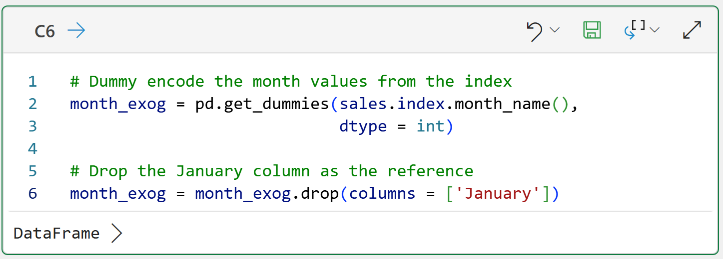
NOTE - While the code above is shown in Python in Excel, it is identical in any other technology (e.g., Jupyter Notebooks).
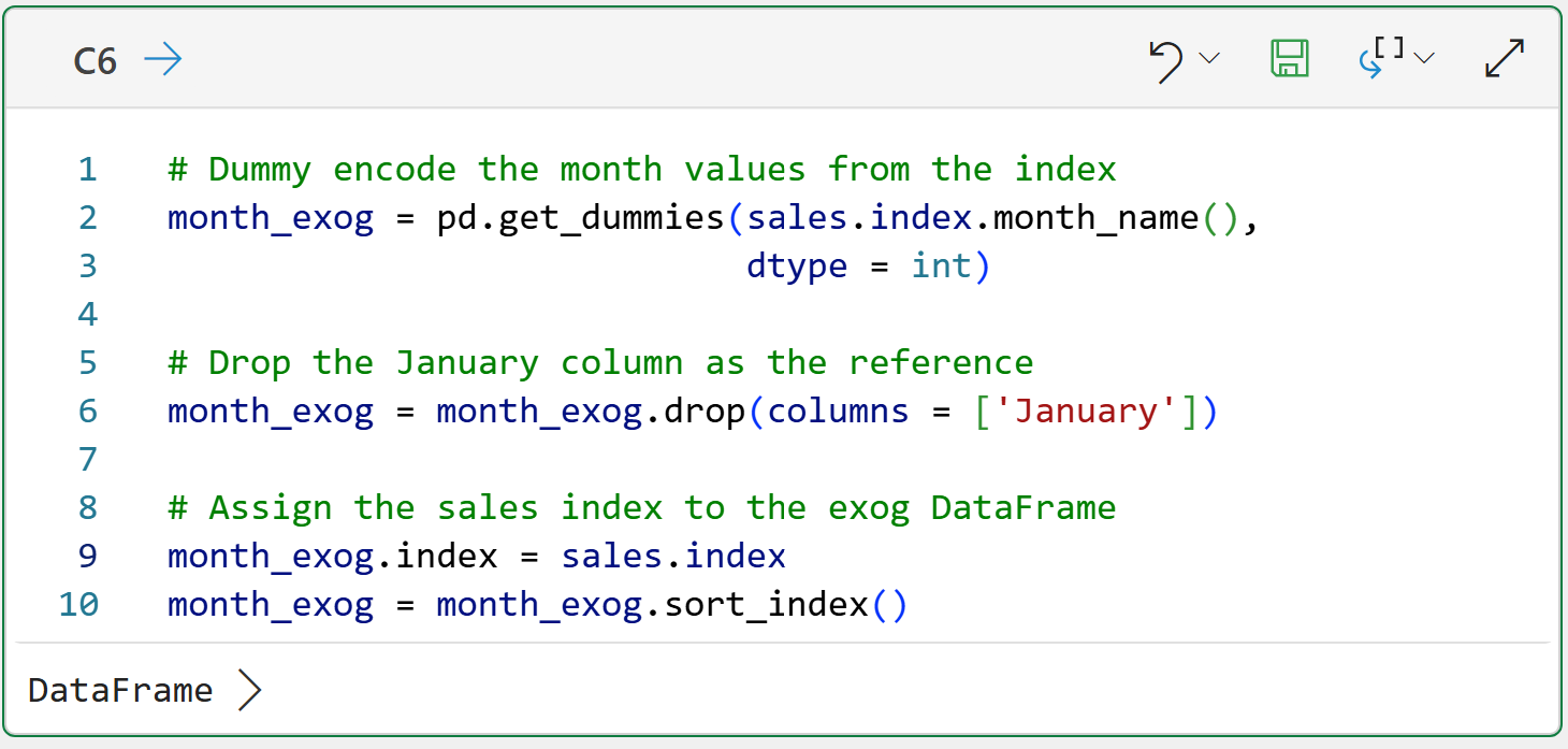
While the DataFrame created from the Python formulas in cell C6 will work as-is, changing the month_exog's index to match the index for the sales DataFrame will make the next step easier:
BTW - If you're new to Python, my book Python in Excel Step-by-Step will teach you the foundation you need for analytics fast.
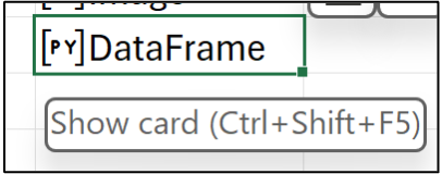
After running the Python formula above, it's a good idea to check out the DataFrame's card by hovering your mouse over the [PY] in cell C6 and clicking:
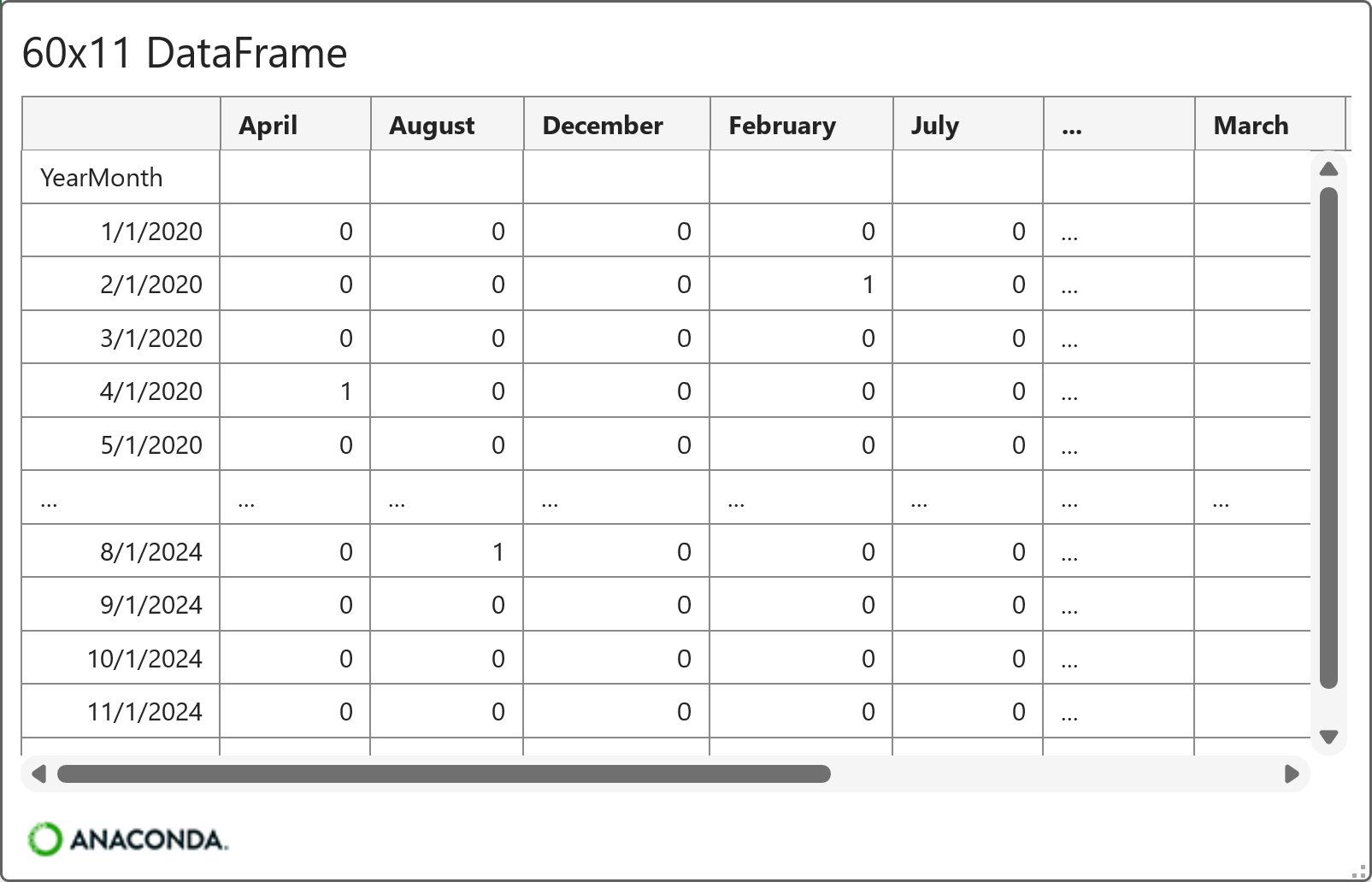
You can see in the image above that the month_exog DataFrame is now indexed by dates (i.e., YearMonth), just like the sales DataFrame.
Splitting the Data
Part 4 of this tutorial series explains the why and how of splitting your time-series data for testing. In Part 6, you learned how to split the data using the YearMonth index.
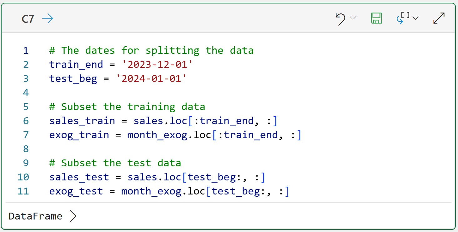
Since the month_exog DataFrame contains all the data, it must also be split into training and test datasets before the ARIMA model can be built (i.e., trained). The following adds a couple of lines of code to what you learned in Part 6:
With the data split into training and test datasets, it's time to tune an ARIMA model using the month name exogenous features.
Tuning the Model
Part 6 of the tutorial series taught you how to tune ARIMA models using a grid search. Once again, the code from Part 6 can be used as a base with two small, but critical, tweaks:
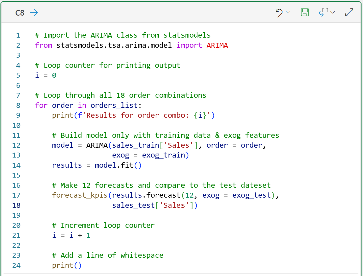
In the code above, lines 13 and 17 achieve the following goals:
The ARIMA model is provided with the exog_train DataFrame from which to learn (hopefully) the seasonal impacts on the sales data.
The exog_test DataFrame is required to make forecasts because the ARIMA model was trained using exog_train (i.e., you can't make forecasts without the month name features).
As you learned in Part 6, the code above explores 18 different combinations of ARIMA component values and evaluates each by comparing model forecasts to the sales_test actual target values.
The Results
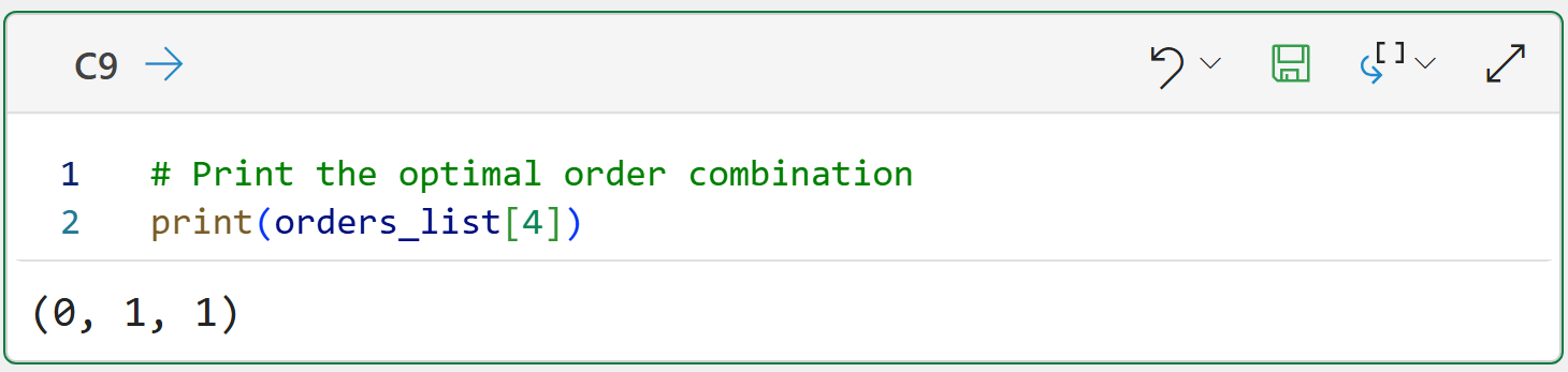
The output of cell C8 is a list of KPIs for each combo of ARIMA component values. Searching the list reveals the following as the optimal combination:
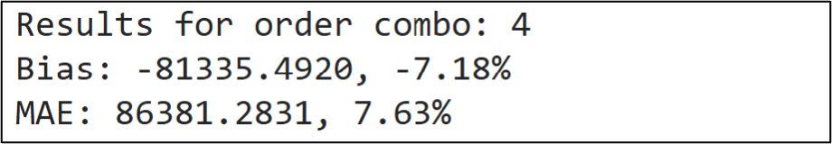
Now, compare the above with the results from Part 6:
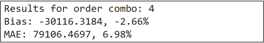
Coincidentally, the optimal combination is the same. However, the KPIs clearly show that forecast quality declined when the exogenous features were added.
In predictive analytics, the process of creating features to build better models is known as feature engineering. Feature engineering is one of the most creative and fun aspects of building predictive models.
But, there's a catch.
Most of the time, the features you engineer don't work. This is a great example.
You shouldn't be discouraged by this outcome. This is a normal part of crafting the best predictive models, including your forecasting models.
If you're wondering what the next steps might be in a real-world project, a good place to start would be experimenting with a Seasonal AutoRegressive Integrated Moving Average with eXogenous regressors (SARIMAX) model.
As you might have guessed from the name, SARIMAX is an extension of ARIMA and offers a more sophisticated way of dealing with seasonality. And the statsmodels library includes SARIMAX.
This Week’s Book
I was recently asked about introductory books on data analysis. This is a great book that I recommend to professionals (including managers, BTW) for getting started with data analysis:

Now here's what you may find interesting. The professional who asked for a recommendation is a Data Analyst at an IT organization. This is something I see all the time.
Many Data Analysts spend very little time actually analyzing data. Instead, they spend most of their time building/maintaining dashboards and reports. Data analysis is a different skill.
That's it for this week.
Next week's newsletter will cover Copilot in Excel AI prompts for building ARIMA models.
Stay healthy and happy data sleuthing!

Dave Langer
Whenever you're ready, here are 3 ways I can help you:
1 - The future of Microsoft Excel forecasting is unleashing the power of machine learning using Python in Excel. Do you want to be part of the future? Order my book on Amazon.
2 - Are you new to data analysis? My Visual Analysis with Python online course will teach you the fundamentals you need - fast. No complex math required, and Copilot in Excel AI prompts are included!
3 - Cluster Analysis with Python: Most of the world's data is unlabeled and can't be used for predictive models. This is where my self-paced online course teaches you how to extract insights from your unlabeled data. Copilot in Excel AI prompts are included!