
Join 1,000s of professionals who are building real-world skills for better forecasts with Microsoft Excel.
Issue #51 - Forecasting with ARIMA Part 6:
Your First Model
This Week’s Tutorial
The previous tutorials in this series provided you with the necessary background for crafting useful (i.e., accurate) forecasting models. If you're new to this tutorial series, you can access all previous tutorials from my website (scroll to the bottom of the page).
In this tutorial, you will craft the first iteration of an ARIMA time series forecasting model using the mighty statsmodels package and Python in Excel.
(BTW - Other than the code for loading the data from Excel, the Python is the same for any other technology like Jupyter notebooks.)
If you would like to follow along with today's tutorial (highly recommended), you will need to download the SalesTimeSeries.xlsx file from the newsletter's GitHub repository.
ARIMA Components
As you learned in previous tutorials in this series, ARIMA forecasting models can be thought of as being built from three components:
The autoregressive (AR) component, where lagged data is used to help craft a more accurate model.
The differencing component that is used to make time series data stationary.
A moving average (MA) component, where it is like an autoregressive model of the errors.
These three components are typically referred to as p, d, and q in the academic literature, and the Python statsmodels library adheres to this naming convention.
Now here's the interesting thing.
As you learned in previous tutorials, you can use various values for each of these components:
Using p = 3 means the autoregressive component will use three target lags.
Using d = 1 means the differencing component will use first-level differences.
Using q = 2 means the moving average component will use two error lags.
The above component values can be abbreviated as (3, 1, 2) and specify the ARIMA model's order.
However, it's basically impossible to know which component values will yield the most accurate results for any given time series. So, a common strategy is to try various combinations of component values to find the one that works best (i.e., the optimal one).
In predictive analytics, this process is known as model tuning.
Setting Up the Tuning
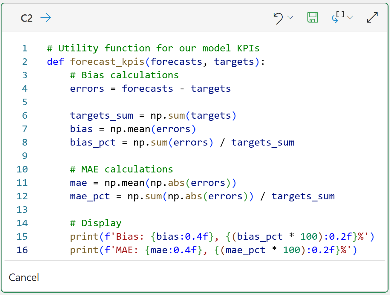
First, as covered in Part 5, we need a Python function that computes our error metrics so we can evaluate each combination of component values.
For brevity, I won't repeat all the steps covered in Part 5. I will simply show the Python in Excel code that calculates the bias and mean absolute error (MAE) KPIs:
BTW - If you're new to Python, my book Python in Excel Step-by-Step will teach you the foundation you need for analytics fast.
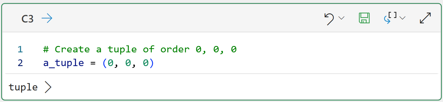
Next, we need a way to provide the statsmodels package with the component values (i.e., the order) we would like to use to train the ARIMA model from the data.
The statsmodels package uses Python tuples to store the model's order:
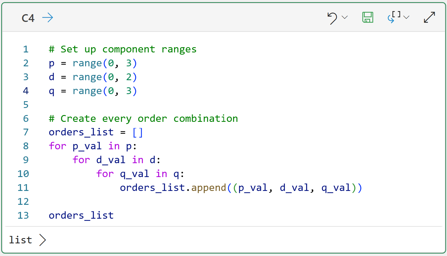
Since we know that we need to try out various orders to find the optimal set of component values, one strategy is to create a list of tuples containing every possible combination. Here's some guidance for this strategy:
In general, it's a good idea to limit the values of p and q to 0, 1, and 2.
Similarly, it's a good idea to limit the values of d to 0 and 1
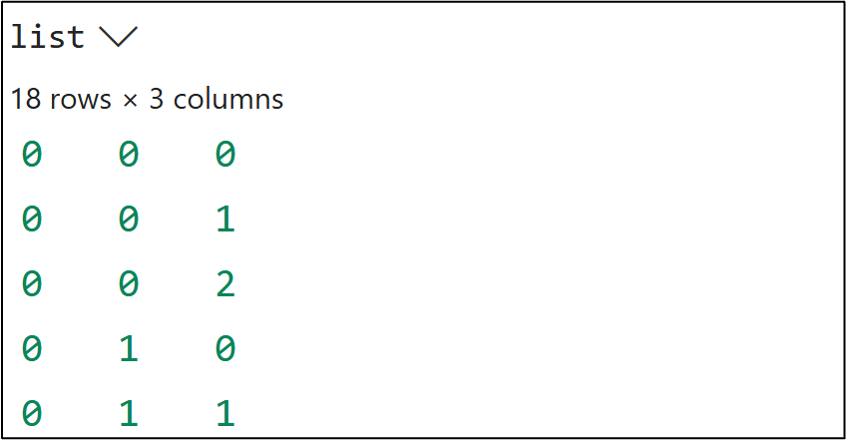
Following the above, we get a total of 18 possible combinations. The following code will create a list of 18 tuples with all the combinations:
And clicking list > at the bottom:
I should mention that you are not limited to the ranges you see in the code above. For example, p = 3 might be optimal for a particular dataset. Tweaking the code above to accommodate scenarios like this is very easy.
With the tuning prepared, the next step is to prepare the data.
Data Preparation
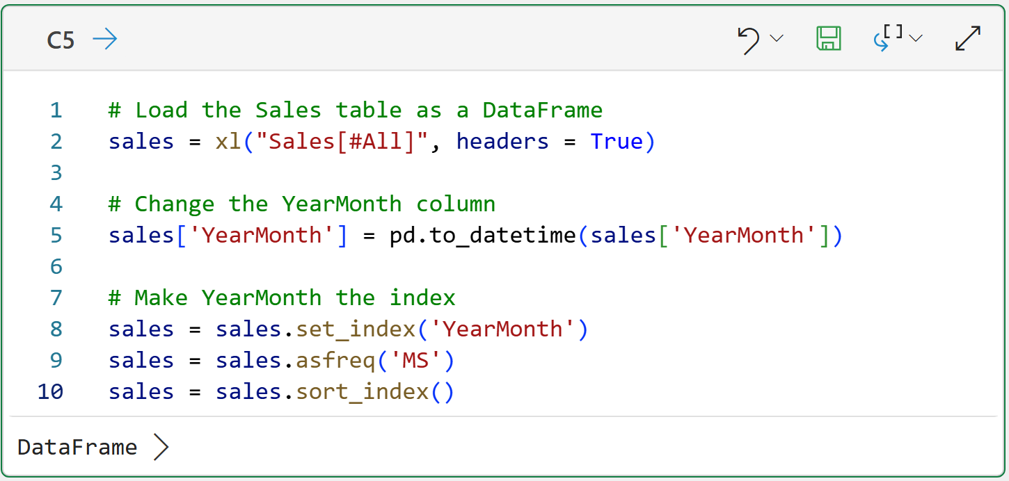
Preparing the Excel Sales table for use with the statsmodels library is covered in Part 2, so I won't repeat the steps in detail here. The following code loads the Sales table as a DataFrame and sets the index to be the YearMonth column:
Next, as covered in Part 4, subsetting the data into training and test datasets will make subsequent code a bit easier:
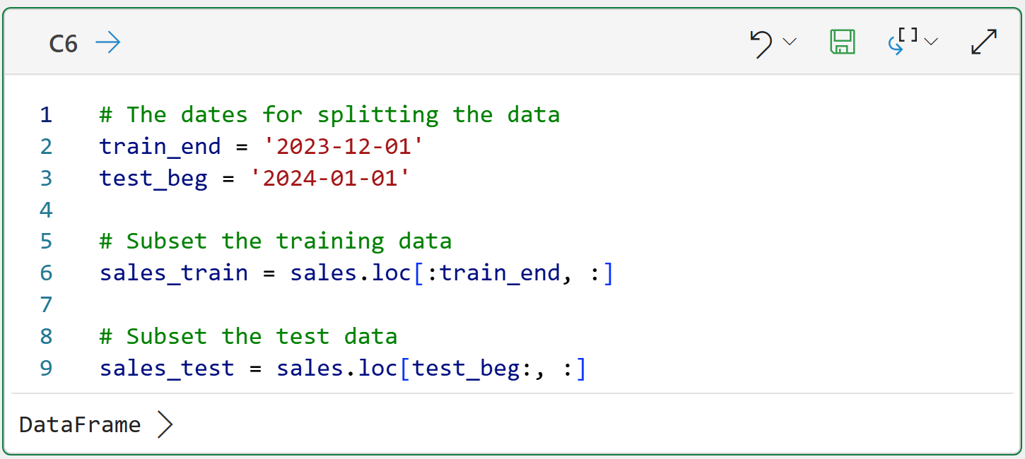
The code above uses loc to subset the data based on the sorted dates:
You can interpret loc[:train_end, :] as, "I want all the rows from the beginning up to train_end and all the columns."
You can interpret loc[test_beg:, :] as, "I want all the rows starting with test_beg through the end and all the columns."
With the data prepared, the next step is to determine the optimal ARIMA order.
Tuning the ARIMA Model
While there are many strategies for finding the optimal ARIMA order for a particular dataset, I'm going to use the simplest strategy - a grid search.
A grid search is a simple brute-force technique that evaluates all possible combinations of values to find the optimal one.
As covered in Part 4, testing your forecasting models is critical for getting the best results. This means you tune your model using only the training dataset.
The following code will build an ARIMA model for every order combination (i.e., it will train a total of 18 models) using only the training dataset:
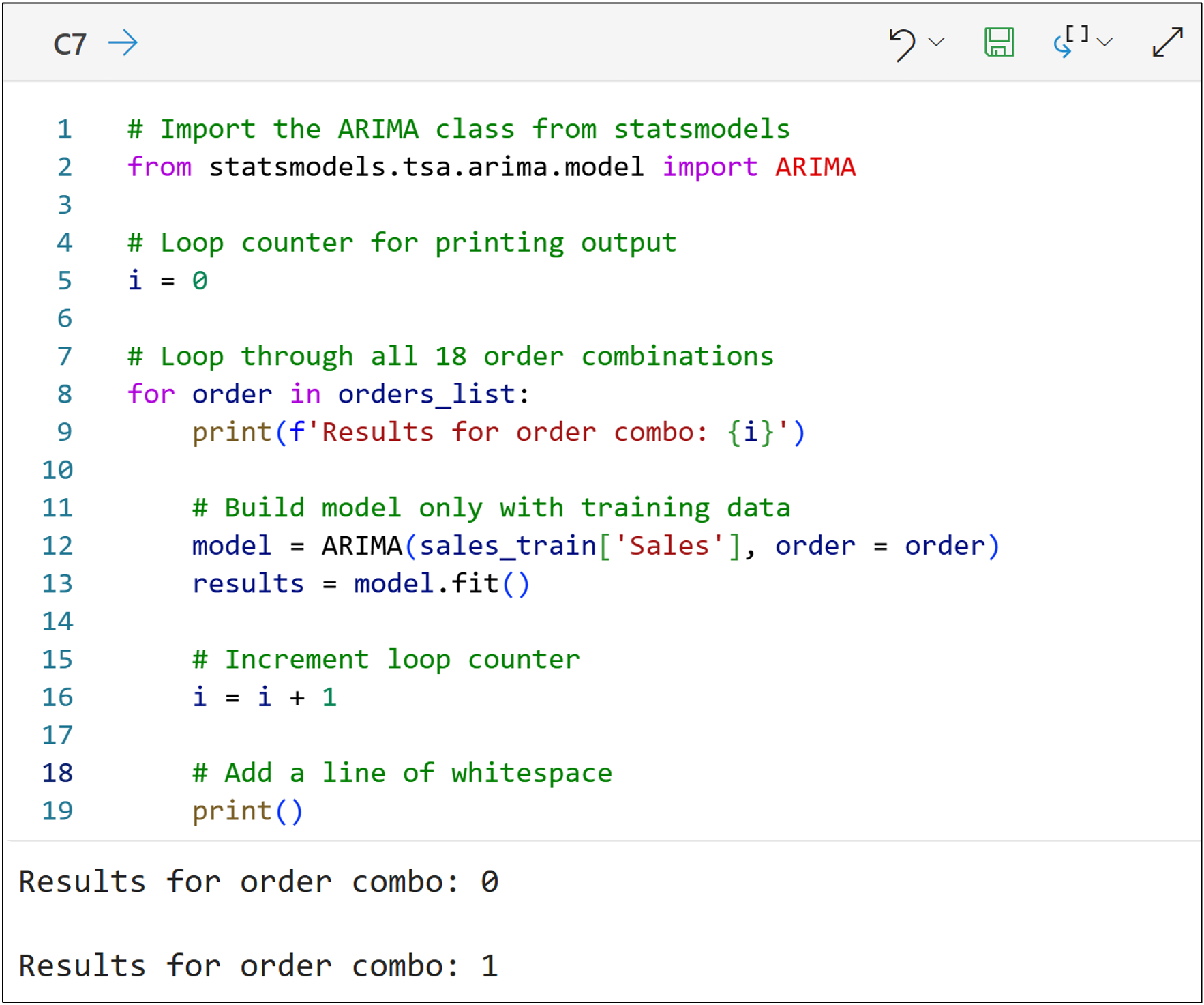
NOTE - The code above is only one of many ways to accomplish the goal. I chose to write the code this way for teaching purposes (e.g., to make it as clear as possible rather than efficient).
A couple of things to note about the code above:
Think of line 12 as specifying the data and the order of the ARIMA model.
Think of line 13 as telling the model to train the model from the data.
In order to evaluate which of the 18 order combinations is optimal for the training data, the following code makes forecasts for 2024 (i.e., 12 months of forecasts) and compares them to the test dataset to simulate the future:
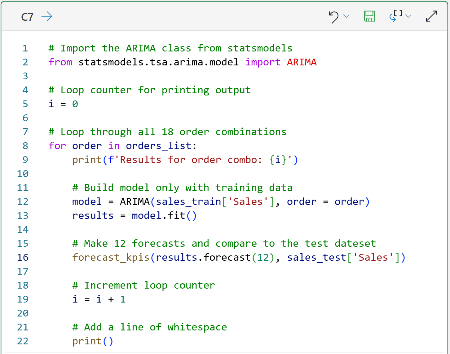
The magic happens in line 16, where two things are happening with this line of code:
Each ARIMA model is asked to make 12 forecasts into the future (i.e., 2024) using the training data and the order combination.
These 12 forecasts are compared to the actual target values of the test dataset, and the KPIs are calculated
The final step of this tutorial is looking at the results.
Choosing the Optimal Order Combination
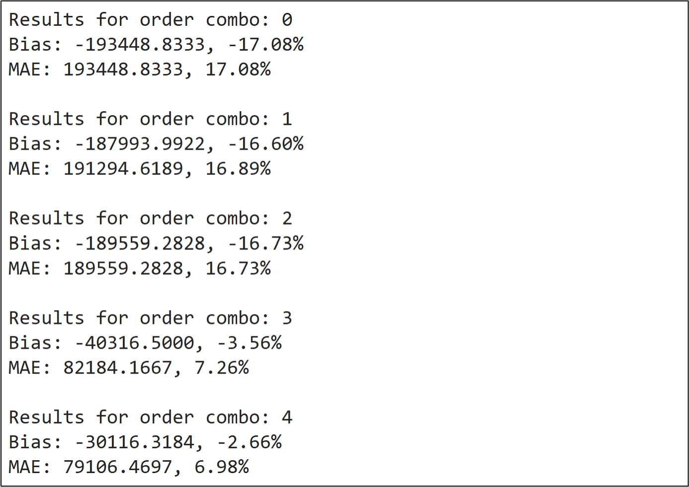
The following shows some of the output of the Python formula in cell C7:
NOTE - Once again, I wrote the code this way for teaching purposes. You could certainly write code to automate this more compared to what you see in this tutorial.
Finding the optimal order combination is simply a matter of scrolling through the 18 combinations to find the lowest bias and MAE values:
Combination 4 looks quite promising, but there are a couple of things to call out:
Combination 11 produces the same KPI scores.
Combination 16 produces slightly lower bias and slightly higher MAE.
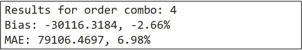
All three of these order combinations are reasonable choices. To keep things simple, I will use combination 4 as the example:
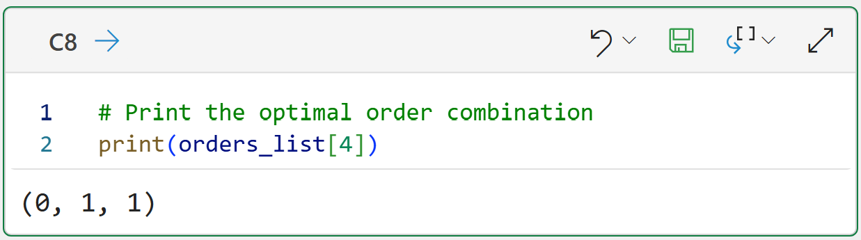
Given the training dataset, the optimal ARIMA model is of order (0, 1, 1):
There are no lagged values used in the autoregressive component.
The training targets are differenced to address stationarity.
A single lagged value is used for the moving average component.
Here's how you should think about the results.
First, the optimal order combination, on average, forecasts values that are too low. Specifically, 2.66% too low.
Second, the optimal order combination, on average, forecasts values that are off by $79,106.
As the forecaster, you can use these values to set expectations with your business stakeholders and also evaluate if your forecasting model will help improve decision-making.
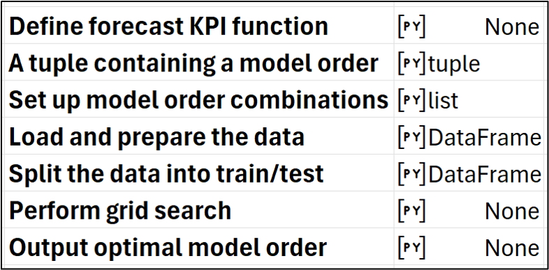
Also, here's how my Python Code worksheet looks after writing all the Python code:
This Week’s Book
Many traditional forecasting models (e.g., ARIMA) are based on statistical principles/techniques. If you want to learn more about statistics, this is a great book for an easy introduction:

Jim Frost is a master at making statistics intuitive and accessible to any professional. If you can't tell, I just love this book.
That's it for this week.
Next week's newsletter will demonstrate how to incorporate seasonality in the quest for an optimal ARIMA model.
Stay healthy and happy data sleuthing!

Dave Langer
Whenever you're ready, here are 3 ways I can help you:
1 - The future of Microsoft Excel forecasting is unleashing the power of machine learning using Python in Excel. Do you want to be part of the future? Order my book on Amazon.
2 - Are you new to data analysis? My Visual Analysis with Python online course will teach you the fundamentals you need - fast. No complex math required, and Copilot in Excel AI prompts are included!
3 - Cluster Analysis with Python: Most of the world's data is unlabeled and can't be used for predictive models. This is where my self-paced online course teaches you how to extract insights from your unlabeled data. Copilot in Excel AI prompts are included!