
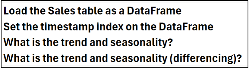
Join 1,000s of professionals who are building real-world skills for better forecasts with Microsoft Excel.
Issue #47 - Forecasting with ARIMA Part 2:
Stationarity & Differencing
This Week’s Tutorial
In Part 1 of this tutorial series, you learned the fundamentals of autoregressive integrated moving average (ARIMA) time series forecasting models.
In particular, you learned how ARIMA models try to uncover the relationships between previous target values (e.g., monthly sales) to build accurate forecasts.
In this week's tutorial, you will learn two critical concepts that enable ARIMA models to learn these relationships - stationarity and differencing.
If you would like to follow along with today's tutorial (highly recommended), you will need to download the SalesTimeSeries.xlsx file from the newsletter's GitHub repository.
BTW - While I'm using Python in Excel in this tutorial series, the code is basically the same if you're using a technology like Jupyter Notebook.
Stationarity Introduction
For ARIMA to learn the patterns in the data sufficiently to create accurate forecasts, those patterns must be stable throughout the time series. In other words, the time series characteristics should not depend on time.
The easiest way to build an intuition is to think about when a time series is not stationary:
When a time series exhibits a trend.
When a time series exhibits seasonality.
In both cases, the target values in the series are time-related (e.g., sales drop in January). For more information on trend and seasonality, check out this previous tutorial.
Take the Sales dataset from the tutorial's Excel workbook as an example:
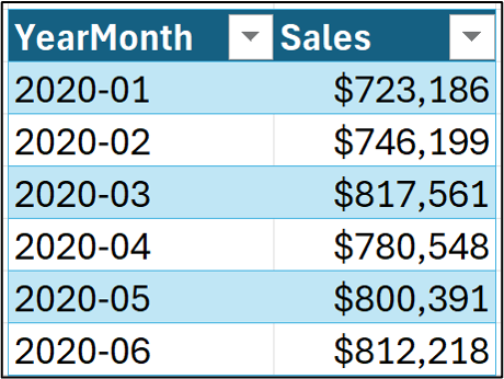
To build a useful ARIMA model to forecast these data, the pattern in the Sales target needs to be stationary (e.g., it has no trend).
The easiest way to do this robustly is to use Season-Trend decomposition using Loess (STL). The statsmodels Python library provides an implementation of STL that can be accessed via Python in Excel.
Loading the Data
When using Python in Excel, it's best to organize your Python formulas (i.e., code) to make writing and maintaining your data goodness easier.
I'm a big fan of putting all my Python formulas in a single worksheet, with the code laid out vertically, step by step. First step is to add a worksheet:

Next, I add comments to my Python worksheets for my own long-term sanity:

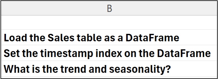
I then place my Excel formulas immediately to the right of each comment. In this case, I would click cell C2 to contain the Python formula to load the Sales table.
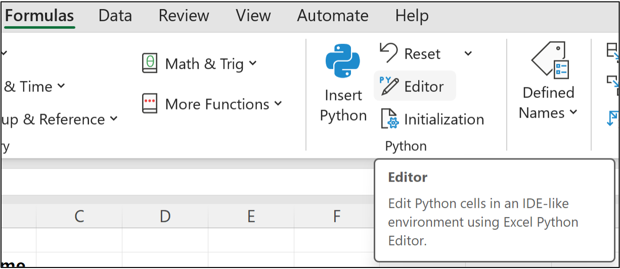
The best way to write Python formulas is to use the new Python Editor, which you can access from the Ribbon:
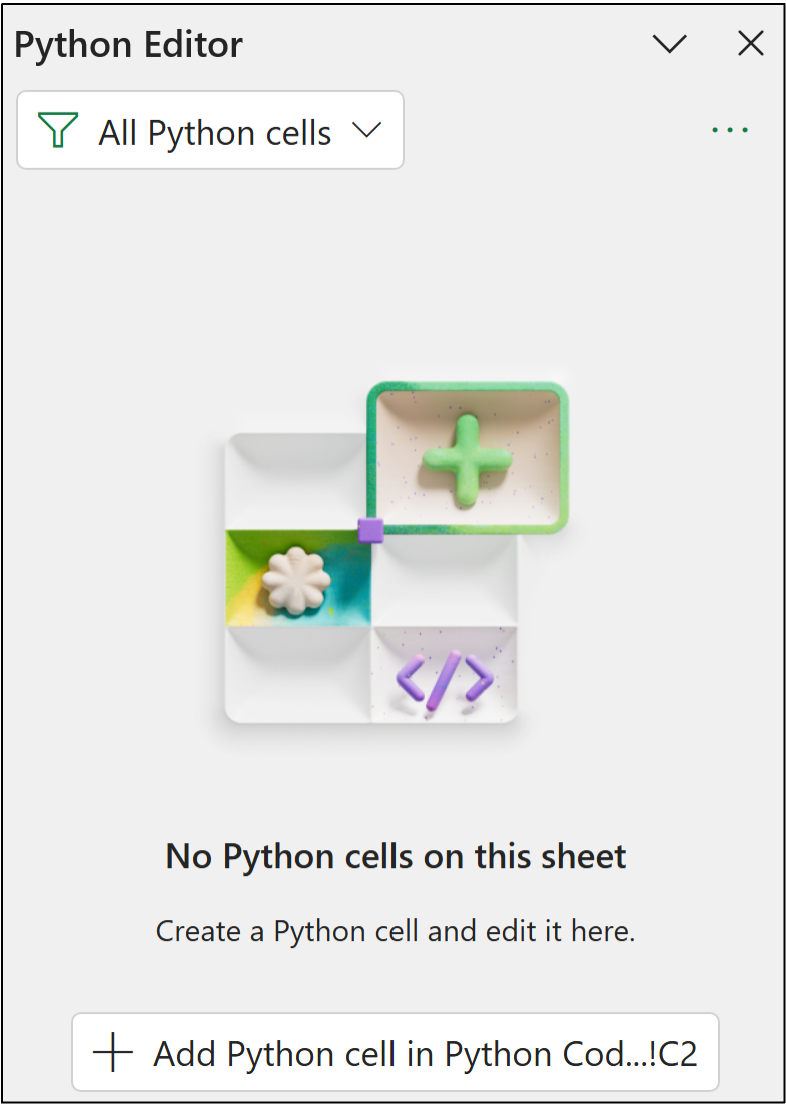
Clicking the Python Editor opens a new pane:
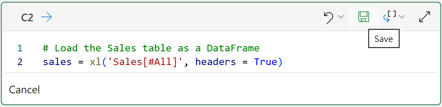
Notice how the button at the bottom of the Python Editor references cell C2? Clicking the button inserts a new Python formula in that cell where you write your code:

The code in the image above loads the Sales table from Excel into a Python DataFrame (i.e., how Python represents entire data tables).
Clicking the disk icon will save (i.e., run) the Python formula:
If you enter the code correctly, you should get a new DataFrame:

Clicking on the > in the Python Editor gives you a preview of the DataFrame:
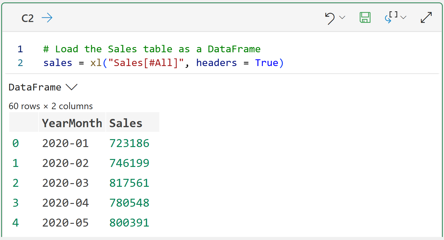
The output above shows 60 rows of data (i.e., 5 years of monthly sales) and two columns: YearMonth and Sales.
BTW - The Python code you see here is specific to Python in Excel. The rest of the Python code in this tutorial is the same regardless of the technology used (e.g., Jupyter Notebook).
Preparing the Data
When working with time series data (e.g., forecasting) using Python in Excel, you usually need to format your DataFrames in a particular way:
Your timestamps have to be recognized by Python.
The DataFrame is indexed by the timestamp.
Python doesn't recognize the YearMonth column as a timestamp because Excel didn't recognize it as a date. However, this is easily fixed by adding another Python formula to the worksheet:
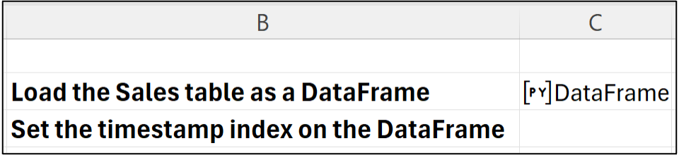
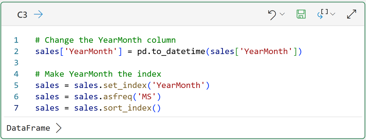
Conceptually, the Python formula in cell C3 sets up the DataFrame to have an index based on the YearMonth column, where each value corresponds to the first day of each month.
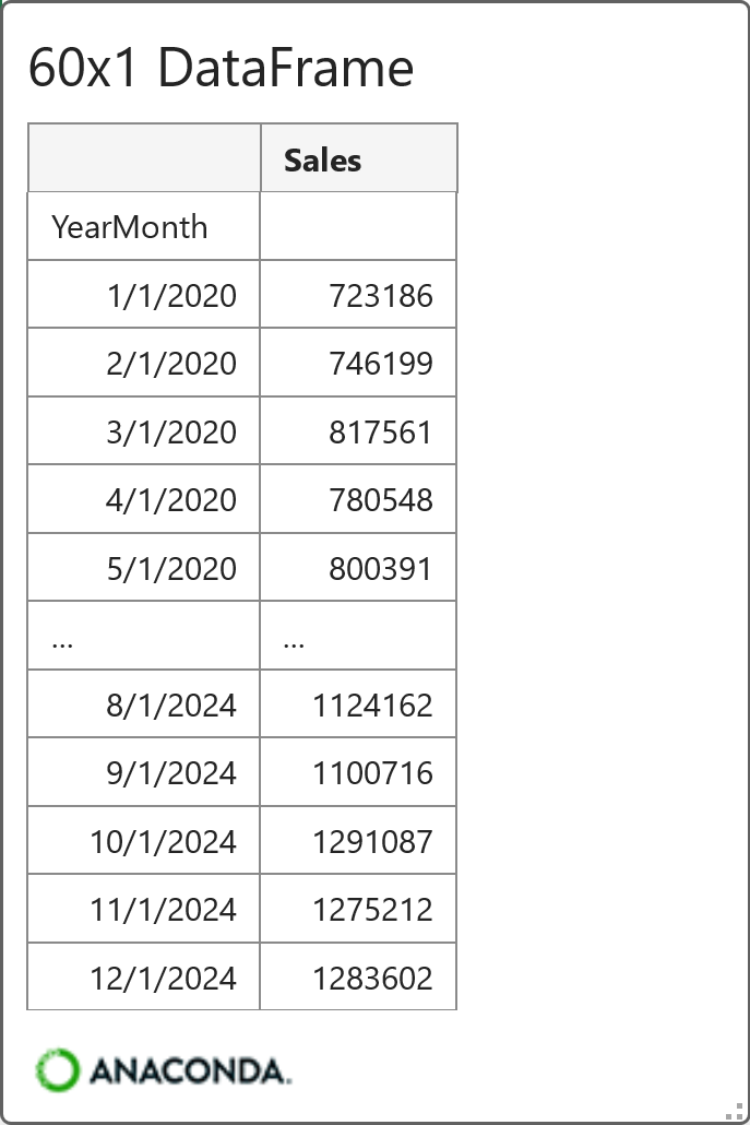
You can think of a DataFrame index as providing a unique identifier for each row in the table. You can see this in action by hovering over the [PY] in cell C3 and clicking on the card:

Excellent!
With the data now prepared, the next step is to see if there's a trend or seasonality.
Detecting Trend and Seasonality
Python in Excel comes with the mighty statsmodels library. Think of statsmodels as a collection of functions that you can use to access powerful tools to build better forecasts.
In many cases, better forecasts are possible than those using native Excel features.
Accessing the power of STL is simple using Python in Excel:
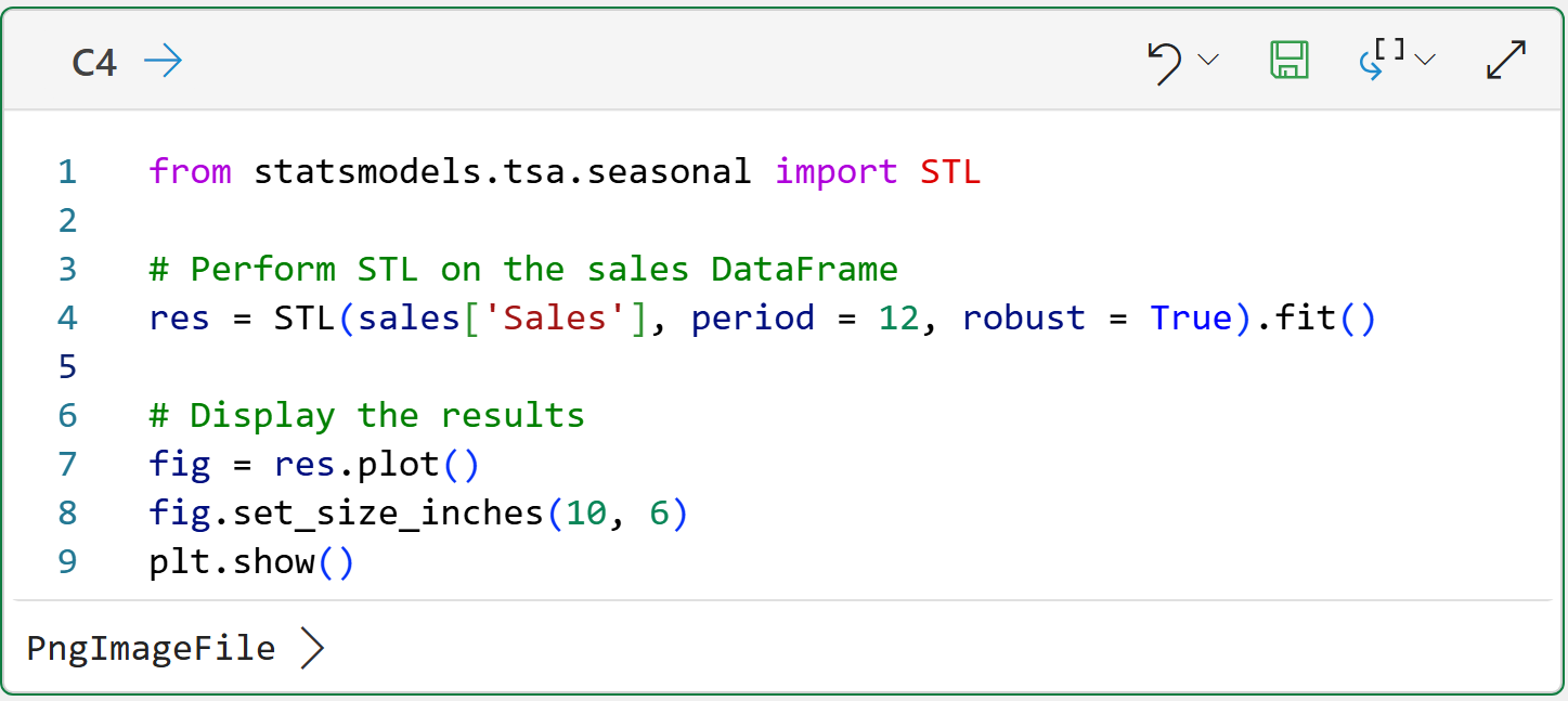
The Python formula in cell C4 tells STL to analyze the Sales column and that the data is monthly (i.e., period = 12). Also, the robust = True tells STL to use a version that is robust to some form of outliers.
The formula also creates a visualization (i.e., plot) of the results for ease of analysis, specifying to create a visual that is 10 inches wide and 6 inches high.
Clicking the > in the Python Editor provides the visual:

The image above clearly shows both trend and seasonality in the Sales dataset. Specifically, you're looking for predictable patterns in the trend and seasonality:
The trend line is straight and increases over time (i.e., it's predictable).
The seasonality shows lower sales every January (i.e., it's predictable).
Stationary data is not predictable, so ARIMA will have a problem with this dataset "as-is."
In cases like this, ARIMA uses a technique known as differencing to eliminate predictable trends and seasonality, thereby arriving at a stationary dataset.
Differencing
As it turns out, there's a simple technique for making a time series dataset stationary: differencing.
Instead of using the raw target values (e.g., the Sales column), you create a new column that is the difference between the two subsequent target values.
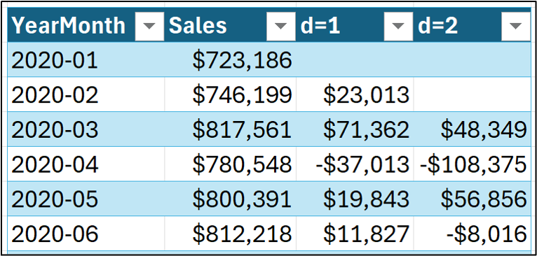
Differencing is often abbreviated as d. Differencing the raw target values is often abbreviated as d=1:
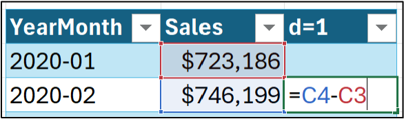
And dragging the formula down the length of the table:
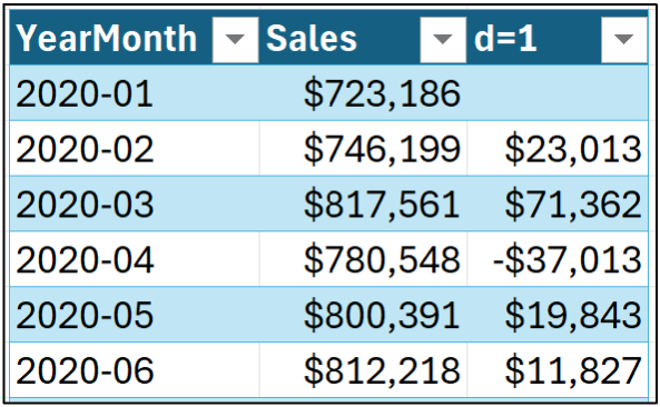
In many situations, using d=1 is enough to get a stationary dataset. However, if needed, ARIMA can use differences of differences (i.e., d=2):
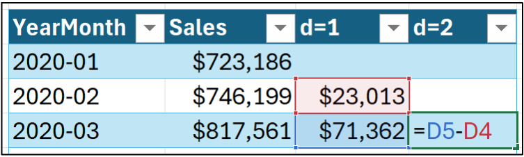
It turns out that d=2 is not common in practice. So, I will stick with d=1 for this tutorial series.
Conceptually, when using differences, ARIMA learns to forecast the change (i.e., the difference) between the targets, not the targets themselves. The predicted changes are then added to the target value to arrive at the final forecast.
Don't worry, as you will see later, the ARIMA model handles differencing and forecasting for you automagically. I'm showing you how to do the differencing in Excel solely for educational purposes.
Differenced Trend and Seasonality
With the differenced columns added to the Sales Excel table, you can then add a Python formula for running the STL on the d=1 column:
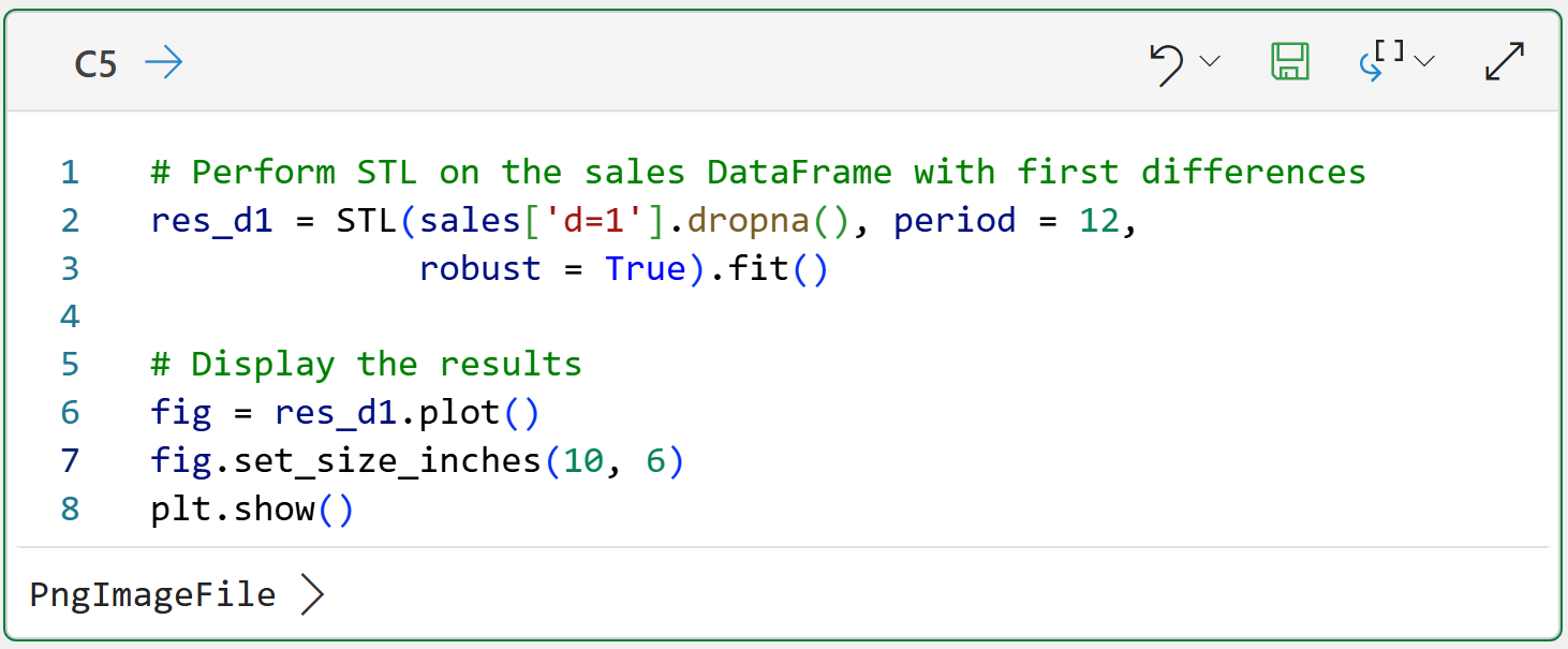
In the code above, the dropna() is necessary because the first cell in the d=1 column is missing. This function drops any missing values before running STL.
Re-running all the Python formulas (which is the default) will load the new differencing columns. Here's the output for cell C5:
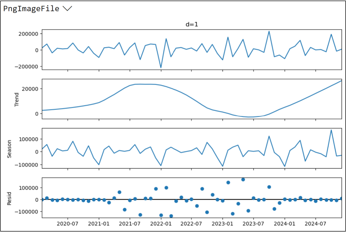
The above image shows that the d=1 data no longer has any predictable trend, so this characteristic of the dataset meets the stationarity requirement.
Unfortunately, differencing did not eliminate the seasonality. In looking at the above STL output, it's easy to see that January still has a predictably low value.
To use ARIMA effectively with this dataset, we'll need a way to handle the seasonality beyond using differencing.
This Week’s Book
When I first read this book years ago, it blew my mind. It showed me that Microsoft Excel was capable of so much more than just PivotTables and charts:

While Python in Excel makes this book obsolete, not everyone has access to it. If this is your situation, then this book will show you how to unleash the power of your data by using Solver to hand-roll your analytics (e.g., logistic regression).
That's it for this week.
Next week's newsletter will cover an essential concept for better ARIMA forecasting: adding features to handle seasonality.
Stay healthy and happy data sleuthing!

Dave Langer
Whenever you're ready, here are 3 ways I can help you:
1 - The future of Microsoft Excel forecasting is unleashing the power of machine learning using Python in Excel. Do you want to be part of the future? Order my book from Amazon.
2 - Are you new to data analysis? My Visual Analysis with Python online course will teach you the fundamentals you need - fast. No complex math required, and Copilot in Excel AI prompts are included!
3 - Cluster Analysis with Python: Most of the world's data is unlabeled and can't be used for predictive models. This is where my self-paced online course teaches you how to extract insights from your unlabeled data. Copilot in Excel AI prompts are included!