
Join 1,000s of professionals who are building real-world skills for better forecasts with Microsoft Excel.
Issue #39 - Forecasting with Excel Part 2:
Detecting Trend & Seasonality
This Week’s Tutorial
The topic of this week's tutorial is detecting trend and seasonality in a time series using out-of-the-box Excel features.
If you're new to this tutorial series, you can check out Part 1 here.
If you would like to follow along with today's tutorial (highly recommended), you will need to download the SalesTimeSeries.xlsx file from the newsletter's GitHub repository.
Your First Time Series Model
The best way to learn data-driven forecasting is to start with simple models and gradually add complexity.
Simple forecasting models are also critical for establishing a forecasting baseline that you use to compare whether a more complex model provides any improvements in decision-making.
In this tutorial, you will learn about one of the simplest baseline forecasting models - the simple moving average.
Here's how a moving average works:
Forecasts are made by taking the average of a fixed number of previous target values.
As the forecaster, you pick how many previous target values to use in the moving average.
Moving averages, I find, are quite intuitive when you see them in action.
Let's assume a 6-month simple moving average. Using the data from the Sales worksheet of the tutorial's Excel workbook:
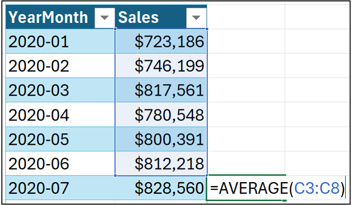
Hitting the <enter> key will create a new column, which can be renamed Forecast. Dragging the formula down the length of the column produces a collection of forecasts:

The next tutorial in this series will evaluate a moving average model in terms of its predictive quality. In this tutorial, we'll use a moving average to help us ascertain the trend of a time series.
A common shorthand notation for moving average models is MA(X), where X represents the number of previous targets used in the average.
The above 6-month moving average model would be abbreviated as MA(6).
Detecting Trend
In this tutorial, you will learn a simple way of detecting a trend in a time series using an MA(12) model. While this technique is easy to implement using out-of-the-box Excel features, it has some issues.
Luckily, since there's Python in Excel, you have access to more powerful tools. A later tutorial will demonstrate the use of the mighty Python statsmodels package.
In the Sales worksheet, delete column D and repeat the moving average modeling process above, but using 12 data points instead:
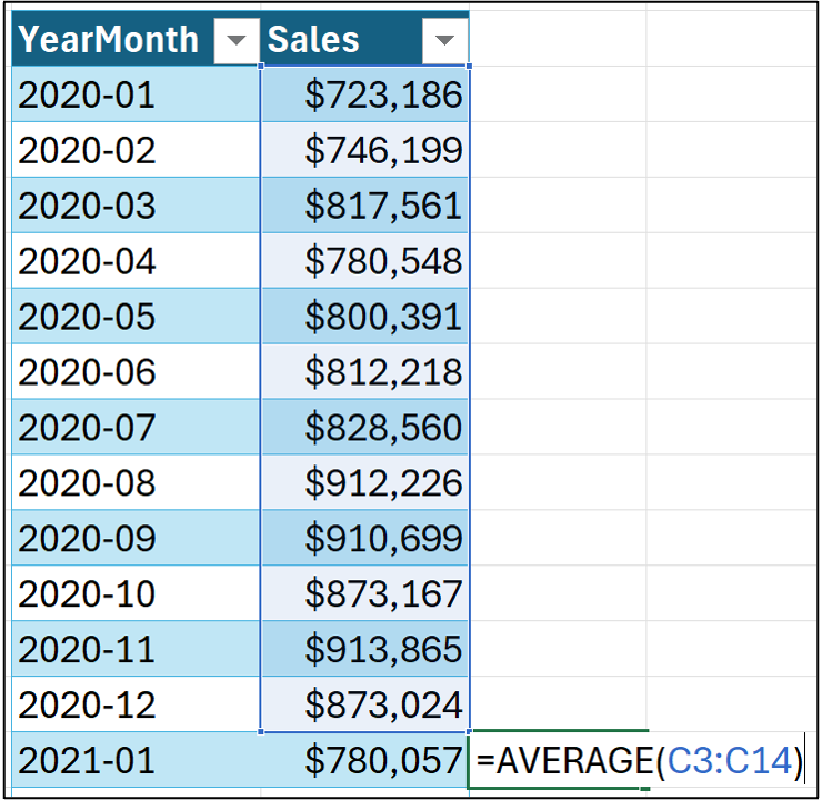
And setting up the column by renaming it to MA(12) and dragging the formula all the way down the length of the table:

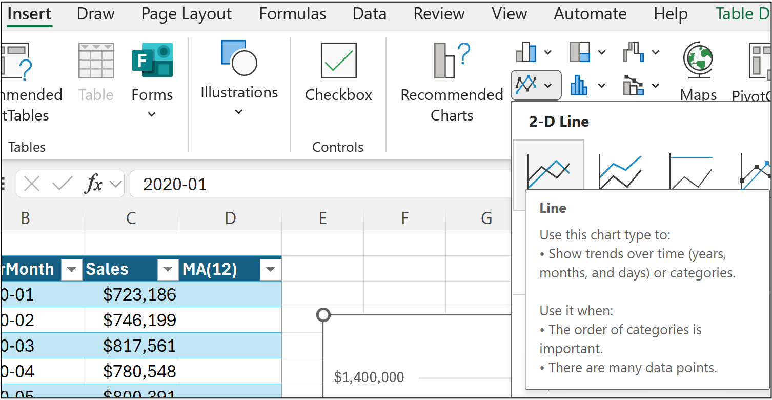
To detect a trend, you now need a line chart of all three columns. First, click on any cell in the Sales table. Then insert a line chart using the Ribbon:
And the line chart tells the story of the trend in the time series:
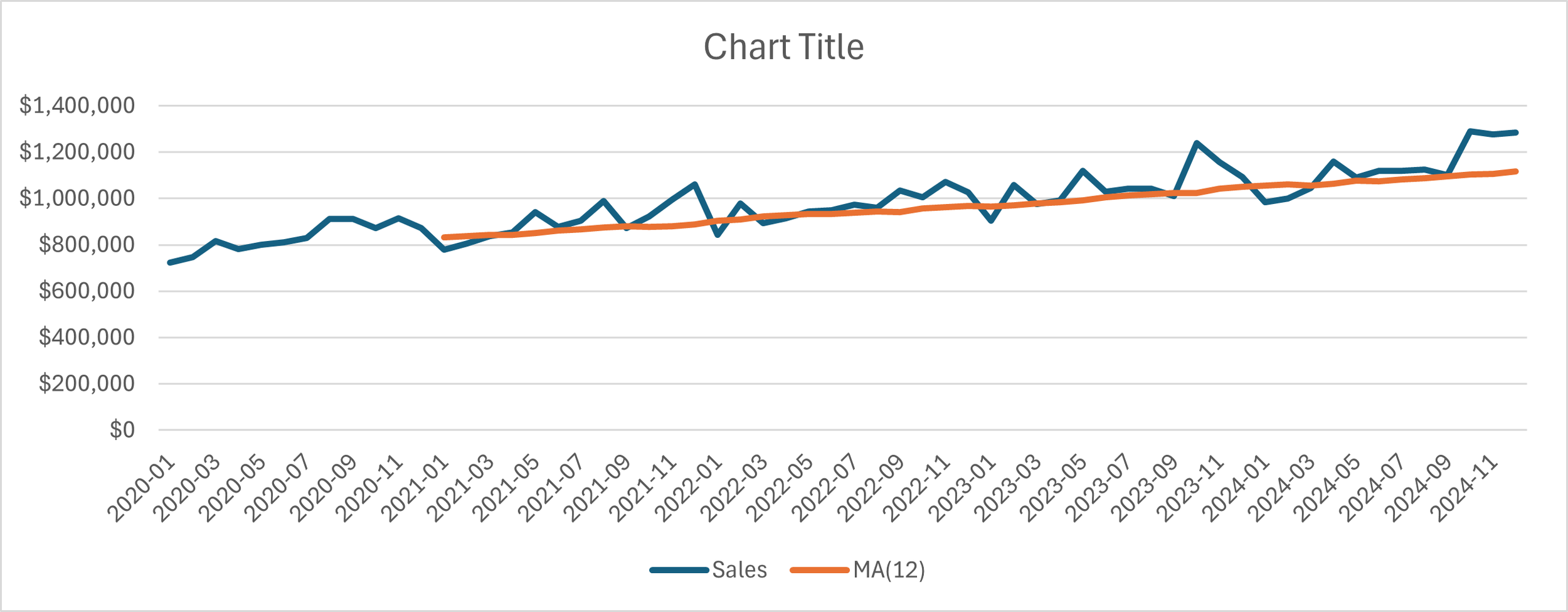
Voila!
The orange MA(12) line clearly has an upward trend.
Detecting Seasonality
As with trends, Python in Excel provides a more sophisticated way of detecting seasonality, which I will cover in a later tutorial.
This week's tutorial will use out-of-the-box features to help you detect if seasonality is present in a time series.
Here's the intuition.
The Sales time series data is at the monthly grain, so the goal is to detect whether certain months tend to have higher target values than others and whether there is a pattern among these higher months.
A Box and Whisker plot (i.e., box plot) can be used to visualize this, but the Sales table isn't set up correctly for Excel box plots. The good news is that setting this up is simple.
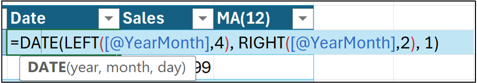
First, we need to create a column that Excel will recognize as dates. Insert a new column named Date between YearMonth and Sales and enter the following formula:
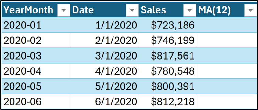
Hitting <enter> populates the column, but you will need to tell Excel to format the column as a date explicitly:
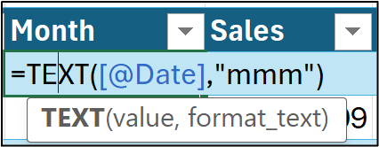
With the Date column created, you can extract the month abbreviations by inserting a Month column and entering the following formula:
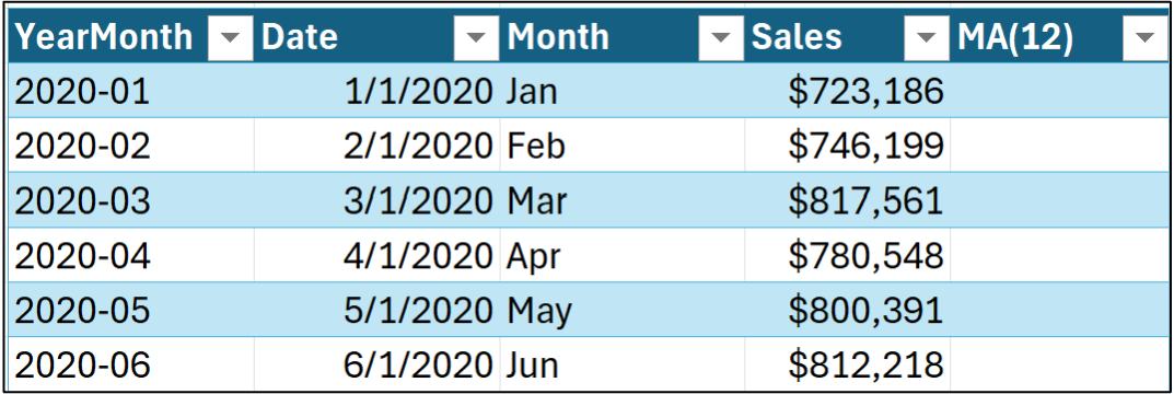
Hitting <enter> populates the column:
With the data set up, click columns D and E in the Sales worksheet:

Now, insert a box plot from the Ribbon:

And here's the resulting visualization:
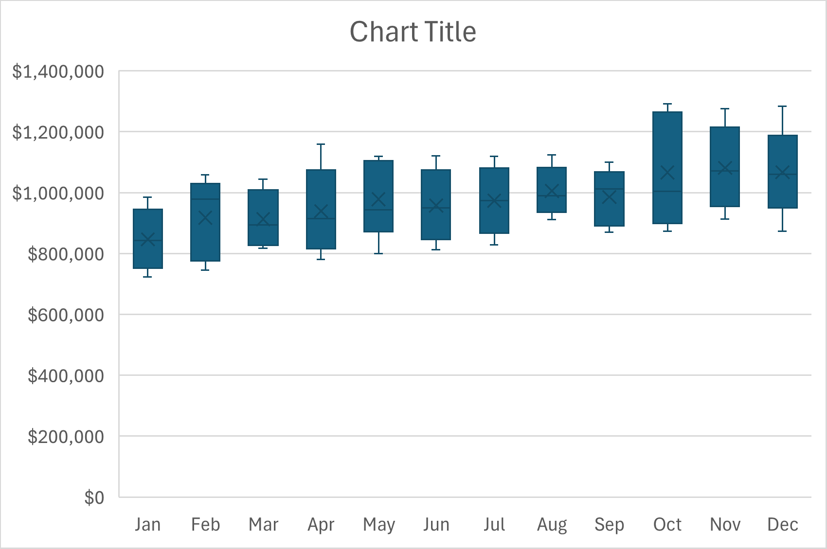
The box plot shows the range (i.e., distribution) of sales values by each month.
For more information on box plots, check out the Wikipedia article.
The box plot indicates that sales are typically higher in the last three months of each year, with a noticeable decline in January. This is likely due to seasonality in the time series
This Week’s Book
All organizations have processes - whether they're formally documented or not. In many cases, these processes are detailed in IT systems (e.g., ERP) and can be mined for powerful insights. This is my favorite book on the subject:

If you're looking to make an impact at work using data, process mining can be a powerful tool in your DIY data science tool belt.
That's it for this week.
Next week's newsletter will introduce you to a critical step for better forecasting using Excel - establishing a forecasting baseline.
Stay healthy and happy data sleuthing!

Dave Langer
Whenever you're ready, here are 3 ways I can help you:
1 - The future of Microsoft Excel forecasting is unleashing the power of machine learning using Python in Excel. Do you want to be part of the future? Order my book on Amazon.
2 - Are you new to data analysis? My Visual Analysis with Python online course will teach you the fundamentals you need - fast. No complex math required, and Copilot in Excel AI prompts are included!
3 - Cluster Analysis with Python: Most of the world's data is unlabeled and can't be used for predictive models. This is where my self-paced online course teaches you how to extract insights from your unlabeled data. Copilot in Excel AI prompts are included!