
Join 1,000s of professionals who are building real-world skills for better forecasts with Microsoft Excel.
Issue #46 - Forecasting with ARIMA Part 1:
The Fundamentals
This Week’s Tutorial
Over the decades, two forecasting models have proven useful to professionals across roles and industries: exponential smoothing and ARIMA.
Exponential smoothing (often called Holt-Winters models) aims to learn the trend and seasonality in your time series data. This type of model is widely used. For example, Microsoft Excel's FORECAST.ETS() function builds these kinds of models.
Autoregressive integrated moving average (ARIMA) models take a different approach to forecasting. ARIMA models aim to capture the optimal relationships in your time series data using historical values.
Knowledge of ARIMA is key for professionals who need more forecasting tools to help the business make better decisions. For example, ARIMA has been extended to handle seasonality (SARIMA) and also to incorporate external factors (SARIMAX).
This tutorial series is designed for any professional. As much as possible, I will take an intuitive approach to understanding how ARIMA models work and how you can apply them to your forecasting problems.
Early tutorials will use Microsoft Excel to illustrate the concepts. Later tutorials will use Python in Excel to build and evaluate ARIMA models. If you don't use Python in Excel, don't worry. The code is 99% the same as using Jupyter Notebooks.
If you would like to follow along with today's tutorial (highly recommended), you will need to download the SalesTimeSeries.xlsx file from the newsletter's GitHub repository.
Forecasting Terminology
Before diving into the first two concepts needed for ARIMA models, I want to establish some common terminology I will use throughout this tutorial series.
First up, what is a time series?
In these tutorials, a time series is defined as a set of measurements collected at regular time intervals. These measurements can include anything, such as sales, demand, advertising spend, claims, etc.
The combination of measurements and a regular time interval is called the data's grain. Consider the following snippet of data from the Sales worksheet of the tutorial Excel workbook:
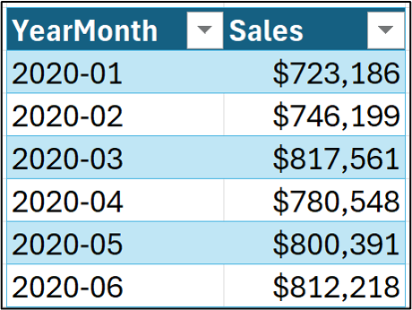
This is a time series dataset at the grain of sales per month.
Most classic (i.e., statistical) time series forecasting techniques, such as ARIMA, work with a single measurement at a time, as in the time series pictured above.
However, a time series can also include additional data. For example:
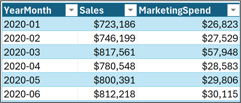
In 2025, state-of-the-art forecasting (e.g., using machine learning) leverages many types of additional data (e.g., promotions, weather, planned expansions, etc.) to improve forecasting.
For example, in the image above, incorporating MarketingSpend data might produce better forecasts than just using Sales data alone.
To keep all of this data straight, I'm going to use the following terminology in this tutorial series:
Timestamps denote the time period for which the data is applicable. In the image above, YearMonth is the data's timestamp.
Targets are the measurement values to be forecasted. In the image above, the Sales column contains the targets.
Features are additional measurements/data that can be used to improve target forecasts. In the example above, MarketingSpend is a feature.
What Are Autoregressive Models?
Conceptually, autoregressive models aren't difficult to understand. These types of forecasting models use previous target values to make predictions.
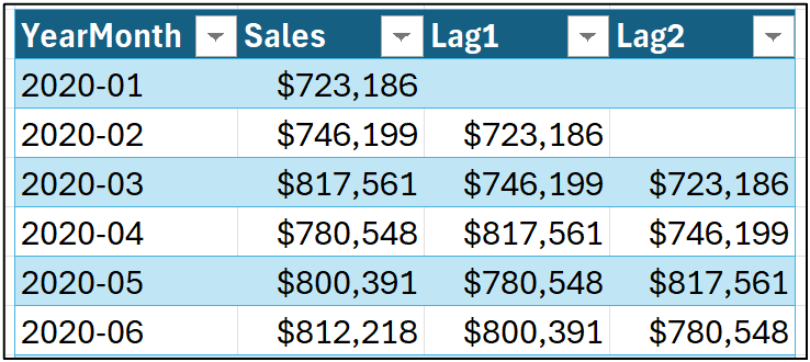
For the purposes of this tutorial series, I will use the term Lags to denote these autoregressive features. For example, consider creating a Lag1 feature that contains the previous target value:

And dragging the formula down the length of the Sales table:

Think of lagged features as mapping to the auto (i.e., "self") portion of autoregressive - you're using previous target values to make the forecast.
The regressive portion of autoregressive can be thought of as building a linear regression model where you use the lagged features to predict the target. For example, using Excel's Analysis ToolPak to create the linear regression model for predicting Sales using Lag1.
BTW - Knowing linear regression is not required for this tutorial, but I do want to demonstrate the concept.
The following screenshot demonstrates the forecasting formula produced by the Analysis ToolPak:
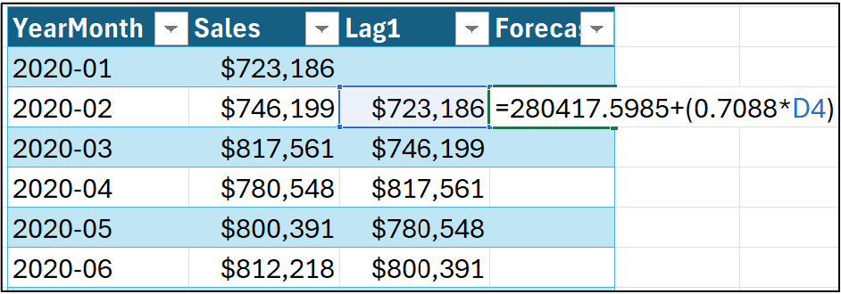
As shown in the image above, the forecasting formula depends on the value of the Lag1 feature. In the formula above, the value of 0.7088 is known as a coefficient.
Dragging the formula down the length of the Sales table:
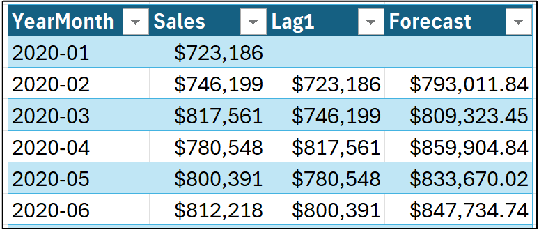
The above autoregressive model is denoted as AR(1) because it goes back one value of the target (i.e., one lag). Here's an example of an AR(2) (i.e. two-lag) model:
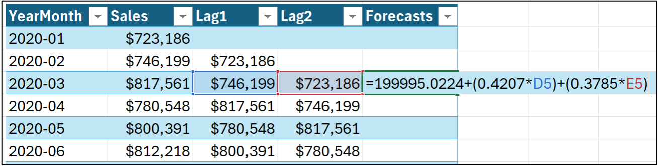
In the image above, the AR(2) model has two coefficients of 0.4207 and 0.3785. There is one coefficient for each lagged feature, and notice that the Lag1 coefficient differs from the AR(1) model. This is normal.

Autoregressive models fit this general pattern. For example, an AR(3) model would have Lag1, Lag2, and Lag3 features with three coefficients.
Model Errors
The key to successful forecasting is to remember this famous saying from the statistician George Box: "All models are wrong, but some are useful."
What this means in practical terms is that every forecasting model you build will be off to some degree. That is, every forecasting model you build will have errors.
In this tutorial series, I will define forecasting errors as the actual target value minus the forecasted (i.e., predicted) value:
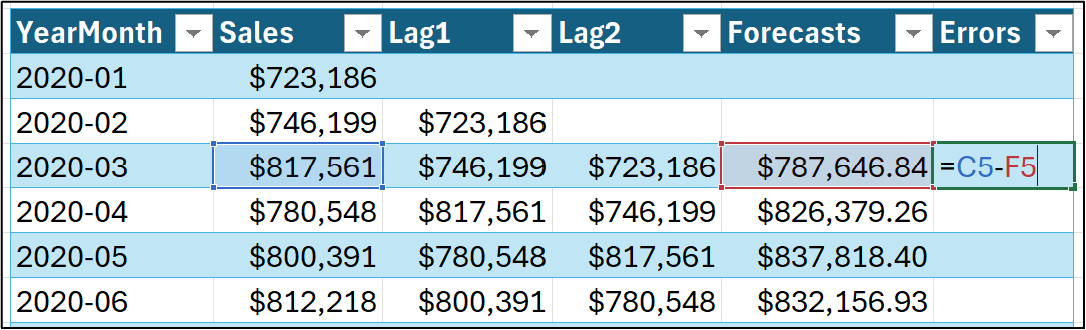
As shown in the image above, a forecasting model's errors are typically positive (the forecast was too low) or negative (the forecast was too high). Only very rarely will the error be zero (the forecast was perfect).
The question is not whether your forecasting model is correct (i.e., it makes perfect predictions), but whether it is accurate enough to support better business decisions.
Later in the tutorial series, you will learn about key performance indicators (KPIs) for evaluating the quality of your forecasting model's predictions.
What Are Moving Averages in ARIMA?
When it comes to ARIMA models, the term "moving average" doesn't align with most people's intuition. For example, this tutorial describes what most people think of when you say, "moving average."
In the case of ARIMA, the moving average is like an autoregressive model of the errors. This deserves a bit of explanation.
So that you know, this will be an intuitive explanation, as the math of how this all works is a bit complicated.
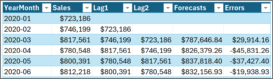
As shown in the image above, it's possible to calculate the error for each model forecast. As shown above, lagged features for the targets can be created; similarly, lagged features for the errors can be crafted.
For example, a moving average with two error lags is denoted MA(2). Conceptually, you can think of these as being features named ErrorLag1 and ErrorLag2. ARIMA then calculates coefficients for each error lag, as you saw earlier for the autoregressive model.
Now, here's where things get really powerful.
Conceptually, ARIMA doesn't estimate all these coefficients separately. Think of ARIMA as estimating all the AR() and MA() coefficients simultaneously to achieve the lowest possible errors.
And you can have different numbers of lags (known as the order) for each. For example:
AR(3) with MA(1)
AR(2) with MA(2)
AR(0) with MA(3)
As you might imagine, picking the right order for AR() and MA() is critical in building the best ARIMA models.
This Week’s Book
Last week, I taught my popular text analytics course at the TDWI Orlando conference. This free online book is one of my favorite ways to get started with Python's powerful Natural Language Toolkit (NLTK):
Mining free-form text data is a powerful way to have more impact at work because many organizations do not allow the uploading of their data to AI services like ChatGPT.
That's it for this week.
Next week's newsletter will cover two critical topics for ARIMA models - stationarity and differencing.
Stay healthy and happy data sleuthing!

Dave Langer
Whenever you're ready, here are 3 ways I can help you:
1 - The future of Microsoft Excel forecasting is unleashing the power of machine learning using Python in Excel. Do you want to be part of the future? Order my book on Amazon.
2 - Are you new to data analysis? My Visual Analysis with Python online course will teach you the fundamentals you need - fast. No complex math required, and Copilot in Excel AI prompts are included!
3 - Cluster Analysis with Python: Most of the world's data is unlabeled and can't be used for predictive models. This is where my self-paced online course teaches you how to extract insights from your unlabeled data. Copilot in Excel AI prompts are included!