
Join 1,000s of professionals who are building real-world skills for better forecasts with Microsoft Excel.
Issue #48 - Forecasting with ARIMA Part 3:
Handling Seasonality
This Week’s Tutorial
In Part 2 of this tutorial series, you learned that ARIMA models require data to be stationary to uncover relationships between target values.
Where stationary data exhibit no predictable trend or seasonality with respect to time.
You also learned that ARIMA uses differencing to transform non-stationary data, aiming to make it stationary.
Lastly, you saw in the Sales dataset that differencing made the trend stationary, but it did not make the seasonality stationary.
In this week's tutorial, you will learn to add features to the dataset to enable the ARIMA model to handle seasonality that wasn't "fixed" by differencing, thereby producing more accurate forecasts.If you would like to follow along with today's tutorial (highly recommended), you will need to download the SalesTimeSeries.xlsx file from the newsletter's GitHub repository.
BTW - While I'm using Python in Excel in this tutorial series, the code is basically the same if you're using a technology like Jupyter Notebook.
The Intuition
As covered in the last tutorial, even after differencing the Sales dataset, predictable seasonality persists (e.g., sales are lower each January).
By default, ARIMA models do not handle predictable seasonality. However, you can enrich the dataset with information about the seasonality that an ARIMA model can use for more accurate forecasts.
In the case of the Sales dataset, that means adding information about the months to the dataset (i.e., adding features to the dataset as discussed in Part 1).
As it turns out, most state-of-the-art forecasting uses additional features to model the ever-increasing complexity of modern business processes.
Endogenous vs Exogenous Features
When it comes to using data to build better forecasts, the features you use fall into one of two categories. While there are technical definitions for the following, for this tutorial series, I will take an intuitive approach:
Endogenous means the feature comes from "inside" the time series target values. For example, a moving average calculated from the time series target values is endogenous.
Exogenous means the features come from "outside" the time series target values. For example, monthly marketing spend is an exogenous feature when monthly sales are the targets.
For the Sales dataset, we need to include exogenous features representing the month of the year so the ARIMA model can learn about seasonality.
However, ARIMA initially did not support exogenous features. Luckily, the statsmodels Python library provides an ARIMA model that can incorporate exogenous features.
So, you can add the months of the year to the Sales dataset, but how do you do that exactly?
Dummy Variables
In many statistical forecasting models, such as ARIMA, you may need to use categorical data to produce the best forecasts.
However, these statistical forecasting models do not understand categorical data. They only understand numeric data.
So, you might be tempted to add a Month feature to the dataset like this:
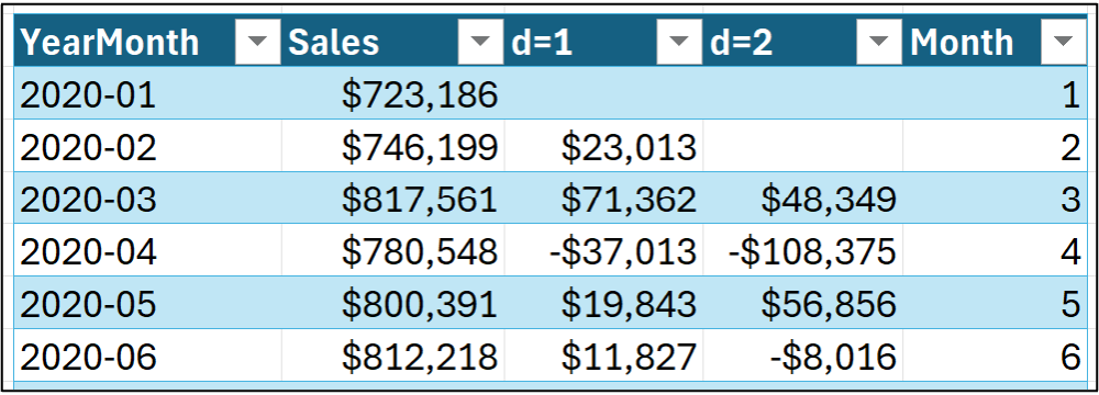
The only problem with representing months this way is that month numbers are not actually numeric in the way a statistical model expects numeric data to behave.
For example, using the dataset shown in the image above, a statistical model would expect that a Month value of 6 is 6 times larger than a Month value of 1. That is, the statistical model would expect June to be six times as large as January.
This is certainly not the case, so we need to represent each month as a category using dummy variables.
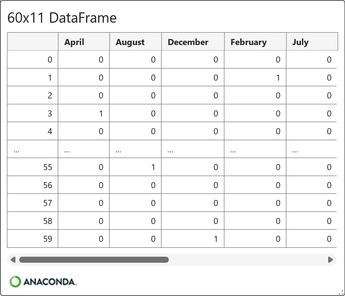
The following features represent the idea behind dummy variables for the first six rows of the Sales dataset (i.e., January through June):
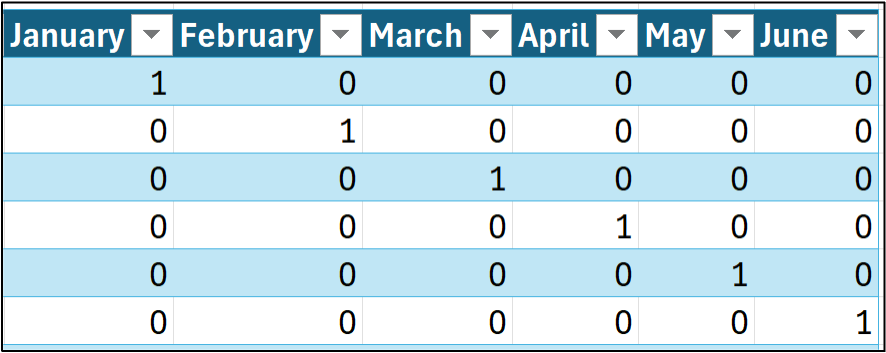
As shown in the image above, each month name (i.e., category) becomes a distinct binary feature. A value of 1 indicates that a category applies to a row of data, while a value of 0 means that it does not.
Given 12 months, 12 binary indicator variables would be created. However, you don't need all 12 to represent the categories.
When you use dummy variables, you only need the number of categories minus one to capture all the information. For example, consider the following, where the January feature has been eliminated:
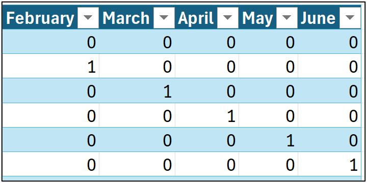
In the image above, take a look at the first row of data. Notice how all the binary indicators are zero? Conceptually, the ARIMA model thinks about the first row like this:
"OK. For this row of data, none of the categorical features are indicated, so this row must be an unnamed category."
The technical name for this unnamed category is reference. In this example, the reference would be January since it is omitted from the data.
The ARIMA model doesn't care which category you use as a reference. It's up to you to pick based on the situation at hand. For this tutorial, I will use January as the reference month.
Preparing the Data
'm not going to go into the steps for preparing the data, as they're covered in Part 2 of this tutorial series. To summarize the steps:
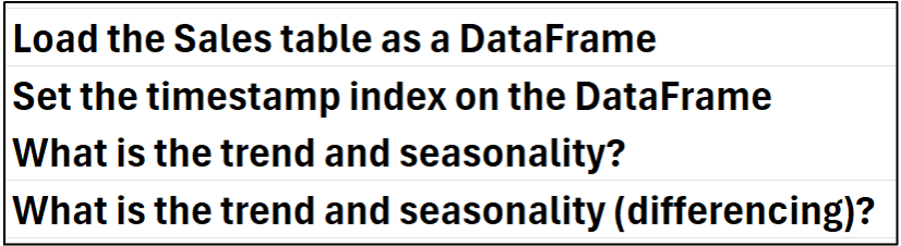
While you could manually create the month dummy variables (i.e., February through December) in Excel, Python provides an easier way.
Dummy Encoding
The process of creating dummy variables is called dummy encoding, and Python provides multiple ways to perform it.
In this tutorial, I'm going to use the pandas library's get_dummies() function. Another option would be to use the OneHotEncoder class from the scikit-learn library.
Per my process, adding the comment to the Python Code worksheet:
Next, adding a Python formula in cell C6:
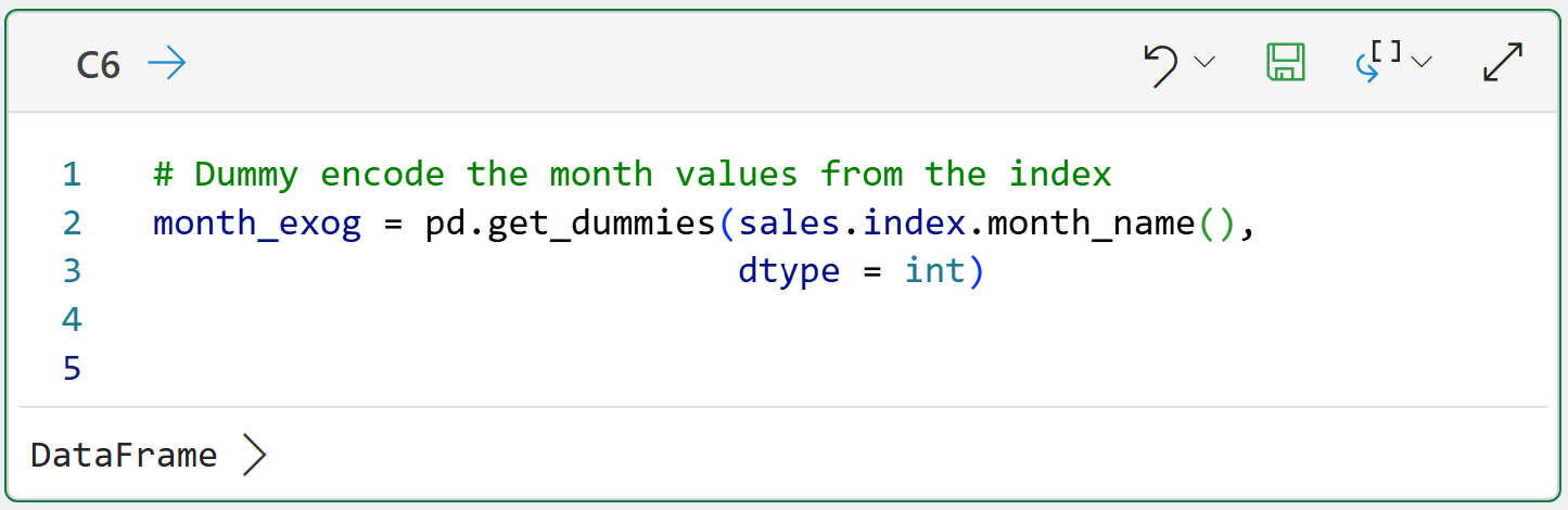
Here's what's going on in the code.
First, the get_dummies() function returns a DataFrame of the encoded features. The code assigns the DataFrame to the month_exog variable (I like to use the exog suffix to denote exogenous features).
The code accesses the index of the sales DataFrame and, since the index is a Datetime object, we can use the month_name() function to return the full month name for each row.
Lastly, the code uses the dtype = int parameter to ensure the data is encoded as 0/1 rather than the default of True/False.
After running the formula, you can easily see the encoded data using the card by hovering your mouse over the [PY] in cell C6 and clicking:

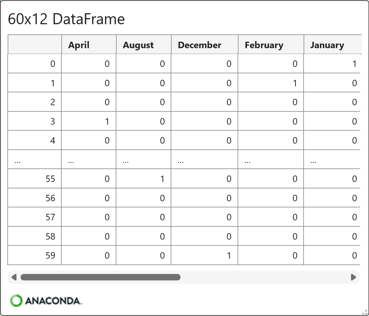
As you can see in the card above, all 12 months were dummy-encoded and arranged in alphabetical order.
The ARIMA model doesn't care about the ordering of the features, but it requires one of the features to be left out as the reference:
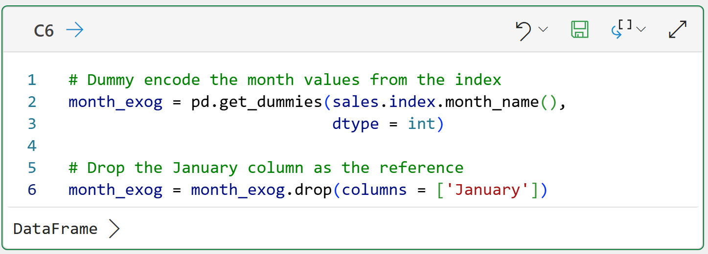
And the card for the final version of the exogenous features:
Outstanding!
By using differencing and the monthly exogenous features, the data is ready for ARIMA modeling.
First, though, I need to drop some caveats on you.
Seasonality Caveats
While using monthly exogenous features isn't technically wrong, it's not optimal. Let me explain why.
When using the monthly exogenous features, the ARIMA model will learn the average difference between each month (e.g., May) and the reference month (i.e., January).
As you know from Part 2 of this tutorial series, January sales tend to be the lowest of all the months of the year. Since January is the reference for the exogenous features, the ARIMA model will learn patterns like:
May sales average 8.4% higher than the reference (i.e., January).
December sales average 12.3% higher than the reference.
BTW - I made those numbers up to illustrate the concept. In a later tutorial, you will learn how to get the coefficients from an ARIMA model.
While the ARIMA model will learn seasonality patterns from the exogenous features, what it learns isn't flexible. Using the bullets above as an example:
The ARIMA model will always add 8.4% to its forecasts in May.
The ARIMA model will always add 12.3% to its forecasts in December.
A more powerful, flexible approach is to use an ARIMA model that models seasonality directly (i.e., no exogenous features required). Not surprisingly, this version is known as seasonal autoregressive integrated moving average (SARIMA).
In general, SARIMA is a better approach to modeling time series data with strong seasonality. I should add that the mighty statsmodels library supports SARIMA with exogenous variables, which is known as SARIMAX.
However, I'm a big believer in the crawl-walk-run approach to learning analytics, so I'm sticking to ARIMA with exogenous variables for this tutorial series.
This Week’s Book
I was recently asked for a statistics book recommendation. The professional doesn't have a math background and was looking for a book that would help them apply statistics without going back to school. This is always the book I recommend:

A psychology professor wrote this book for psychology students, and it is accessible to any professional, regardless of role. Highly recommended.
Oh, and don't let the R part scare you off. In the age of AI, you can have ChatGPT convert the R code to Python for you.
That's it for this week.
Next week's newsletter will cover an essential concept for better ARIMA forecasting: model testing.
Stay healthy and happy data sleuthing!

Dave Langer
Whenever you're ready, here are 3 ways I can help you:
1 - The future of Microsoft Excel forecasting is unleashing the power of machine learning using Python in Excel. Do you want to be part of the future? Order my book on Amazon.
2 - Are you new to data analysis? My Visual Analysis with Python online course will teach you the fundamentals you need - fast. No complex math required, and Copilot in Excel AI prompts are included!
3 - Cluster Analysis with Python: Most of the world's data is unlabeled and can't be used for predictive models. This is where my self-paced online course teaches you how to extract insights from your unlabeled data. Copilot in Excel AI prompts are included!