
Join 1,000s of professionals who are building real-world skills for better forecasts with Microsoft Excel.
Issue #65 - Customer Lifetime Value Part 5:
Predicting CLV
This Week’s Tutorial
RFM segmentation is useful because it turns messy transaction history into something business stakeholders can actually understand.
Recency. Frequency. Monetary value.
Three behavioral signals. Three ways to understand whether a customer is active, loyal, and valuable.
In Part 4, you used these signals to create practical customer segments like:
Champions
At-Risk customers
Recent Customers
That was a huge step forward from using one average CLV number for everyone.
But RFM still has a limitation. It describes customer behavior up to a point in time. What it does not directly answer is this:
Based on what we know about this customer today, how much revenue should we expect from them going forward?
That is the predictive CLV question.
And in this tutorial, you are going to answer it using machine learning in Python in Excel.
BTW - While I will be using Python in Excel for this tutorial, 99+% of the code is the same whether you use Excel, VS Code, or Jupyter Notebook.
Why Two Questions Are Better Than One
The most obvious way to predict CLV is to build a machine learning model that directly predicts future revenue.
That sounds reasonable. But there's a problem.
In many real-world customer datasets, customers will often not buy again during the prediction window. In other words, their future revenue appears to be zero.
Other customers will buy, but will spend very different amounts. So, the model is being asked to learn two very different things at the same time:
Will this customer buy again?
If they do buy again, how much will they spend?
Those are related questions, but they are not the same question. That is why a two-stage predictive CLV is so useful. You break predictive CLV into two smaller problems:
Stage 1 - Will the customer purchase in the next 180 days?
Stage 2 - If the customer is likely to purchase, how much revenue will they generate?
Then you combine the two answers:
Predicted CLV = Purchase Probability × Revenue If Purchase
For example, suppose the stages estimate that a customer has a 40% chance of buying in the next 180 days. If they do buy, the model estimates they will spend $500. The predicted CLV is:
0.40 x $500 = $200
That's the core idea.
A customer can have a high predicted purchase amount but a low probability of making a purchase. Or they can have a modest predicted purchase amount but a very high probability of making a purchase.
Both pieces matter.
What You’ll Build
In this tutorial, you will build a two-stage predictive CLV solution using:
A RandomForestClassifier machine learning (ML) model for Stage 1.
A HistGradientBoostingRegressor ML model for Stage 2.
Raw RFM values as the model inputs (i.e., features).
The customer's actual revenue over the next 180 days.
You will also visualize the final predictions using the mighty plotnine Python library.
To keep this tutorial focused, I am assuming you have already completed the first four steps from Part 2:
Loading the two Excel tables.
Combining them into one DataFrame.
Cleaning the data.
Creating the cleaned transaction-level DataFrame.
However, unlike Part 2, you will not aggregate across the full dataset to create the RFM scores. Instead, you need to separate the data into two parts - one for Stage 1 and one for Stage 2.
An intuitive way to understand why you need to do this is to consider the goal of all this work: accurately predicting how much a customer is likely to spend over the next 180 days, assuming they will purchase again.
You need data to make this possible. At a high level, you need three pieces of data:
A way to characterize the "goodness" of a customer. As you learned in Part 4, you will use RFM scores for this.
For each customer, you need an indicator (i.e., 1/0) of whether they made purchases in the next 180 days.
For customers who purchased in the next 180 days, what was the revenue for each of these customers?
However, you've got a problem.
You don't have a time machine to go 180 days into the future to get the data for the second and third bullets. So, you have to simulate the future using the data you already have.
You use the oldest data for the first bullet, then newer data for the second and third bullets, based on a cutoff date of June 1st, 2011.
Step 1: Import the Libraries
Per my usual, I would strongly suggest placing all your Python in Excel code in a dedicated worksheet (e.g., named Python Code), organized step-by-step vertically.
As you've likely seen from my previous tutorials, I also strongly suggest adding comments to the worksheet for each step:
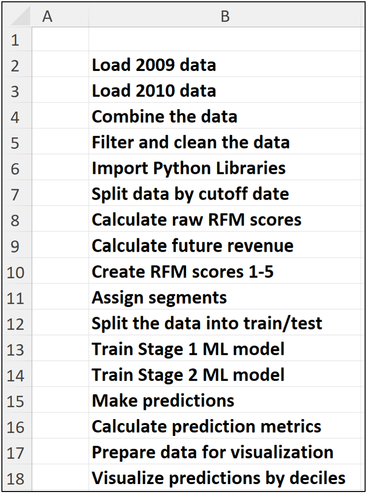
Then, you place your Python formulas to the right of each comment:
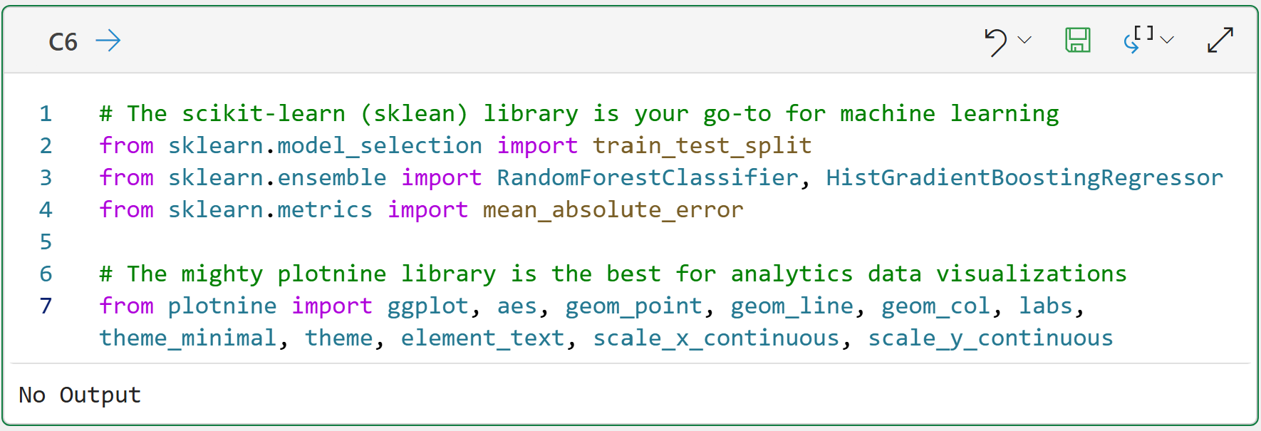
The code above imports a number of useful classes and functions from the scikit-learn (for machine learning) and plotnine (for data visualization) Python libraries that you will use in the tutorial.
If you are new to machine learning, do not let the scikit-learn names scare you.
The RandomForestClassifier builds (i.e., trains) an ML model that makes yes/no (i.e., 1/0) predictions. This model predicts whether a customer will buy within the next 180 days.
The HistGradientBoostingRegressor trains an ML model to predict a numeric value. In this tutorial, it predicts how much revenue a customer is expected to generate if they buy.
That's it.
NOTE - In machine learning, predicting categories like yes/no is called classification, while predicting numeric quantities like dollars is called regression.
Step 2: Create the Cutoff Date and Future Revenue Window
The next step is to define the point in time at which the model must make its prediction. You will use June 1, 2011, as the cutoff date.
The models will use data before June 1, 2011, to predict revenue for the 180 days after the cutoff. Here's the code:
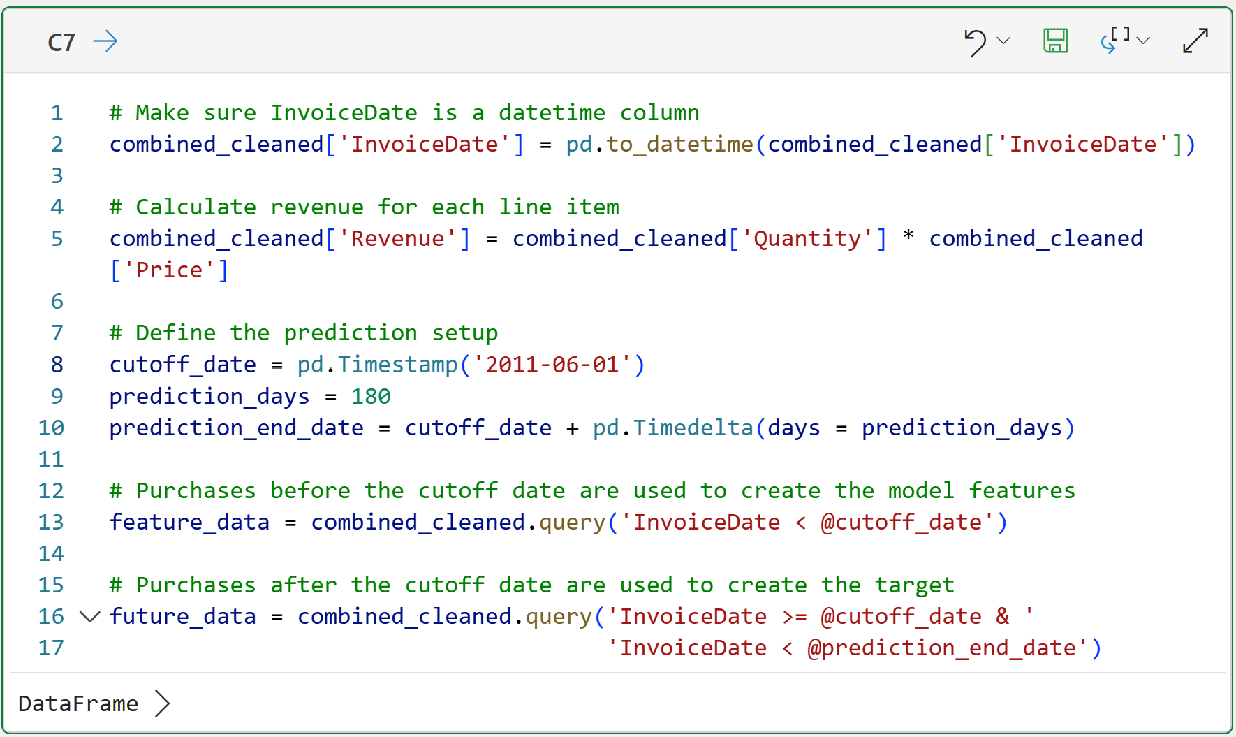
The code above creates two datasets:
feature_data contains customer behavior before the cutoff date.
future_data contains customer behavior during the 180-day prediction window.
The magic happens on lines 13 and 16 of cell C7's code, using the query() method.
If you're familiar with Excel, you can think of these lines of code as operating like Excel filters. If you're familiar with SQL, query() will be second nature to you.
These lines of code illustrate the key difference between the historical CLV approaches you saw in previous tutorials in this series and predictive CLV:
Historical CLV asks: How much has this customer spent?
Predictive CLV asks: Given what we know at a point in time, how much will this customer spend next?
The time split is what makes this analysis predictive.
Part 3: Create the RFM Features Using “Old Data”
The code below is very similar to the code you saw in Part 4, but note that the RFM scores (features) are crafted from feature_data. These data have been filtered to only include customer purchases before June 1st, 2011:
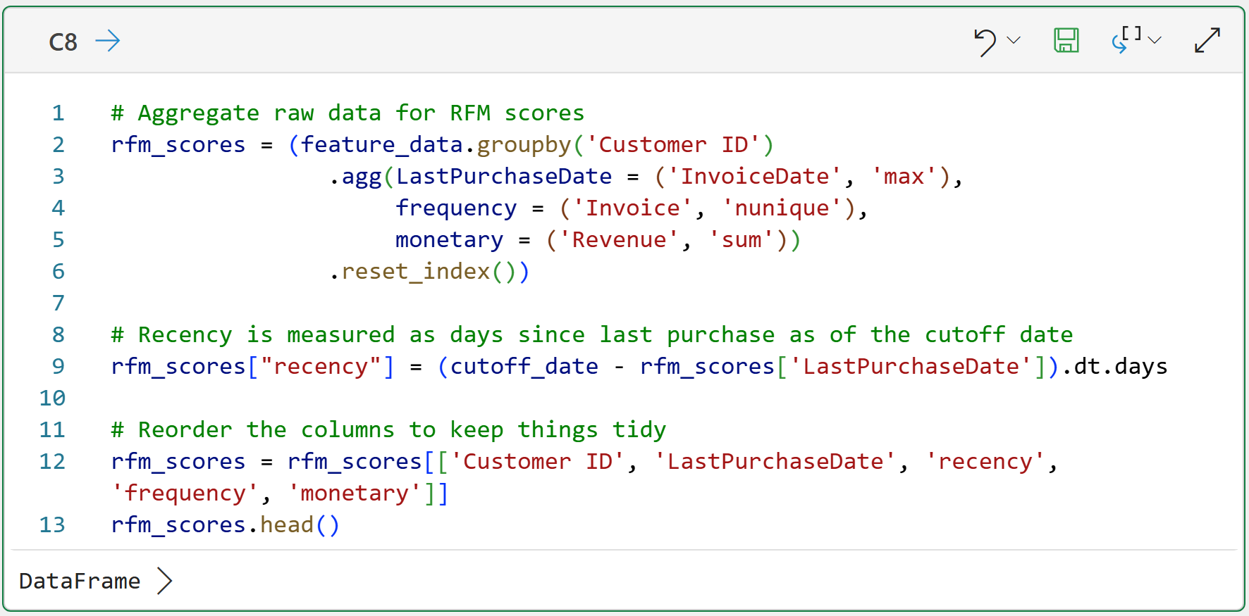
Clicking DataFrame > shows the preview of the rfm_scores:
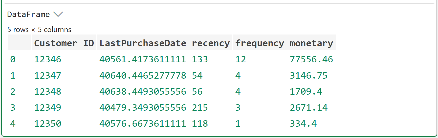
As shown in the output above, the difference now is that the RFM values are calculated as of a specific date (i.e., June 1st, 2011). This is critical.
A customer who bought on May 25, 2011, is very recent as of June 1, 2011. A customer who bought on November 25, 2011, is not allowed to influence the model because that purchase happened after the cutoff date.
This is how you simulate the future using the data you have.
Step 4: Calculate Future Customer Revenue
Next, we need to calculate each customer's revenue during the 180 days after the cutoff date. This is the value the 2nd ML model will learn to predict (i.e., the target).
Make note of how the following code uses future_data (i.e., data after June 1st, 2011) to build the revenue features:
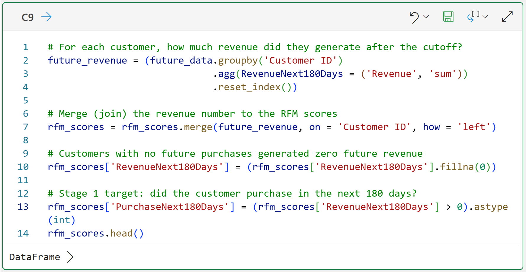
There are a couple of things that are worth some additional explanation in cell C9's code:
The code on line 7 is performing a merge() between rfm_scores and future_revenue. If you're familiar with Excel, this is similar to a VLOOKUP. If you're familiar with SQL, this is a LEFT JOIN.
Because not every customer made future purchases, there will be missing values in the data after the merge. The code on line 10 uses the fillna() method to replace these missing values with zeros.
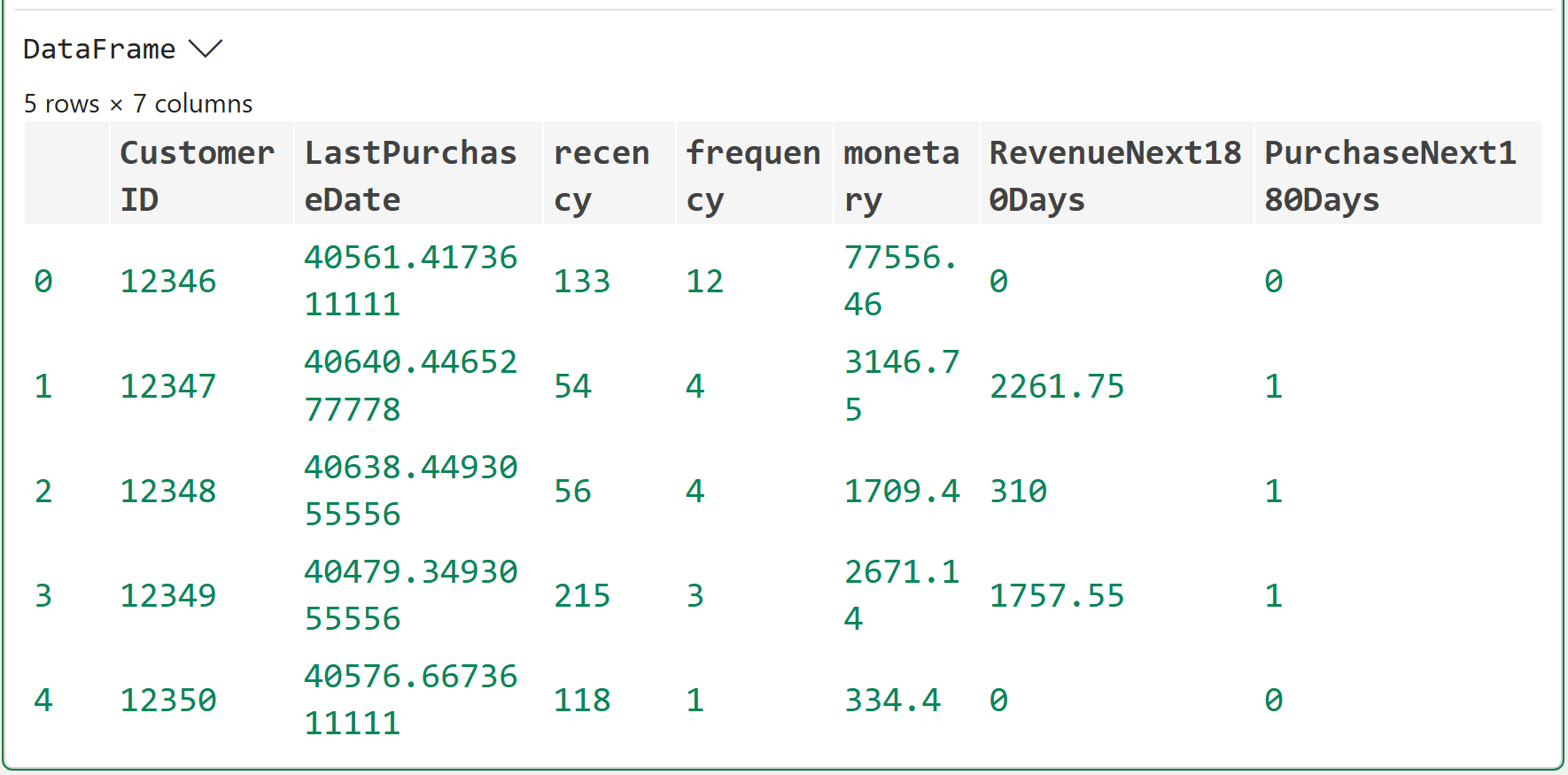
Line 13 then creates a column (i.e., feature) to store a 1/0 value to indicate whether a customer made future purchases.
You now have the dataset needed for two-stage predictive CLV. Each row represents one customer. The customer "goodness" features are:
Recency
Frequency
Monetary
And the ML models will learn to predict the following:
PurchaseNext180Days - Did the customer purchase in the future?
RevenueNext180Days - How much will be purchased in the future?
This is where you move beyond backward-looking RFM to predictive CLV.
Part 5: RFM Scores and Segments
The machine learning model will use the raw RFM values. However, as you learned in Part 4, we still want the RFM segment labels for interpretation.
Why?
Because business stakeholders understand segment names like Champions much better than ML model output columns like PredictedCLV.
The following code recreates the 1-5 RFM scores and assigns segment labels using the same general approach as in Part 4. For brevity, I won't repeat the explanations of the code:
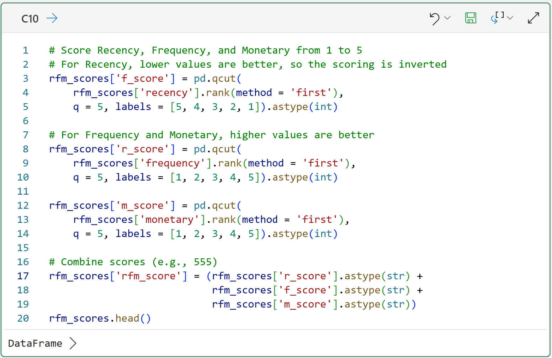
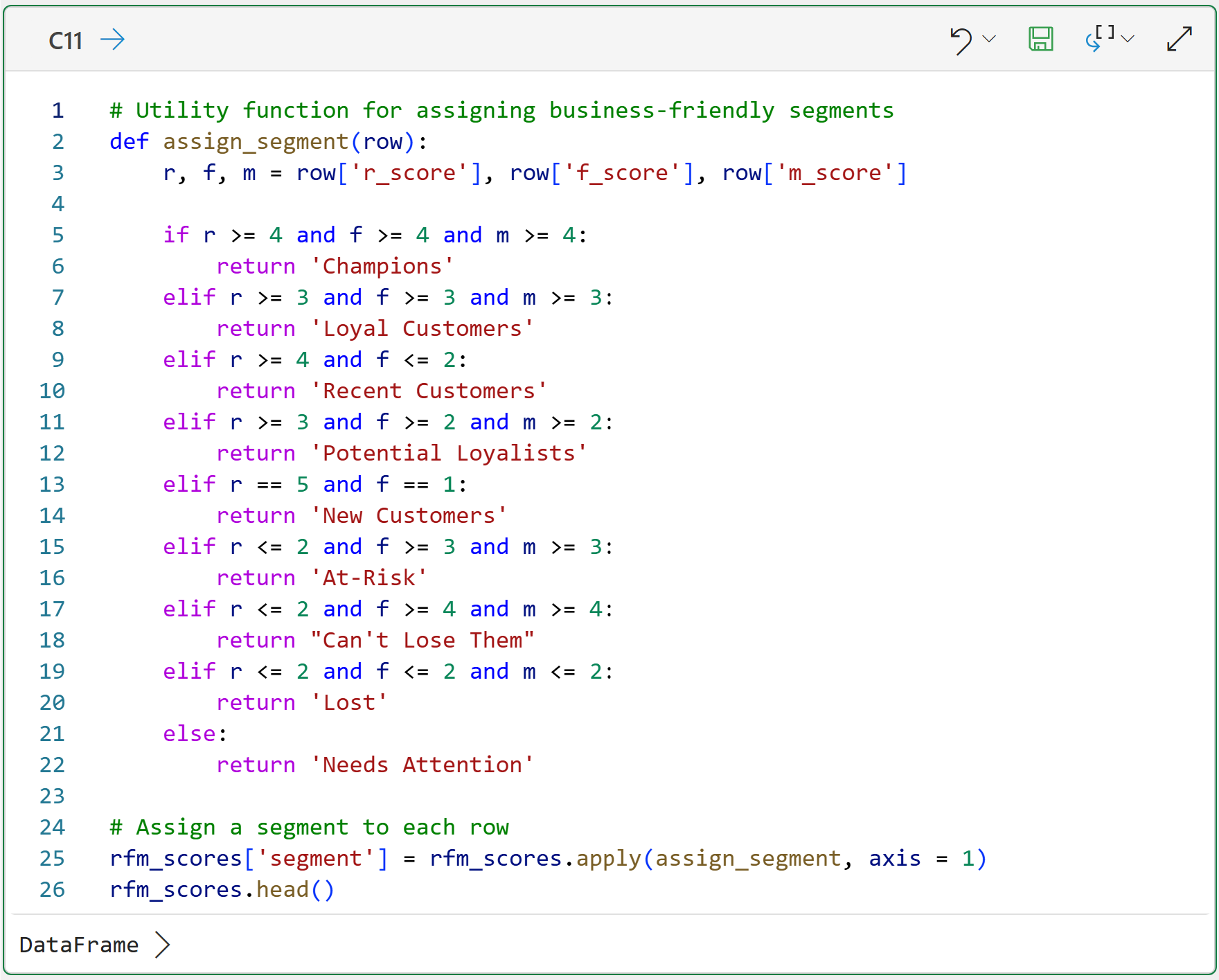
While this tutorial won't use this code, it's included in case you would like to experiment (highly recommended).
Part 6: Split Customers into Training and Test Datasets
Machine learning models are like humans in this regard - you have to test your ML models if you want to know for sure they've learned the things you wanted them to learn.
So, it's common practice to split your data into a training set to train the ML model and a test set to evaluate how well the model learned from the training data.
Here's the code to randomly split the "old" data:
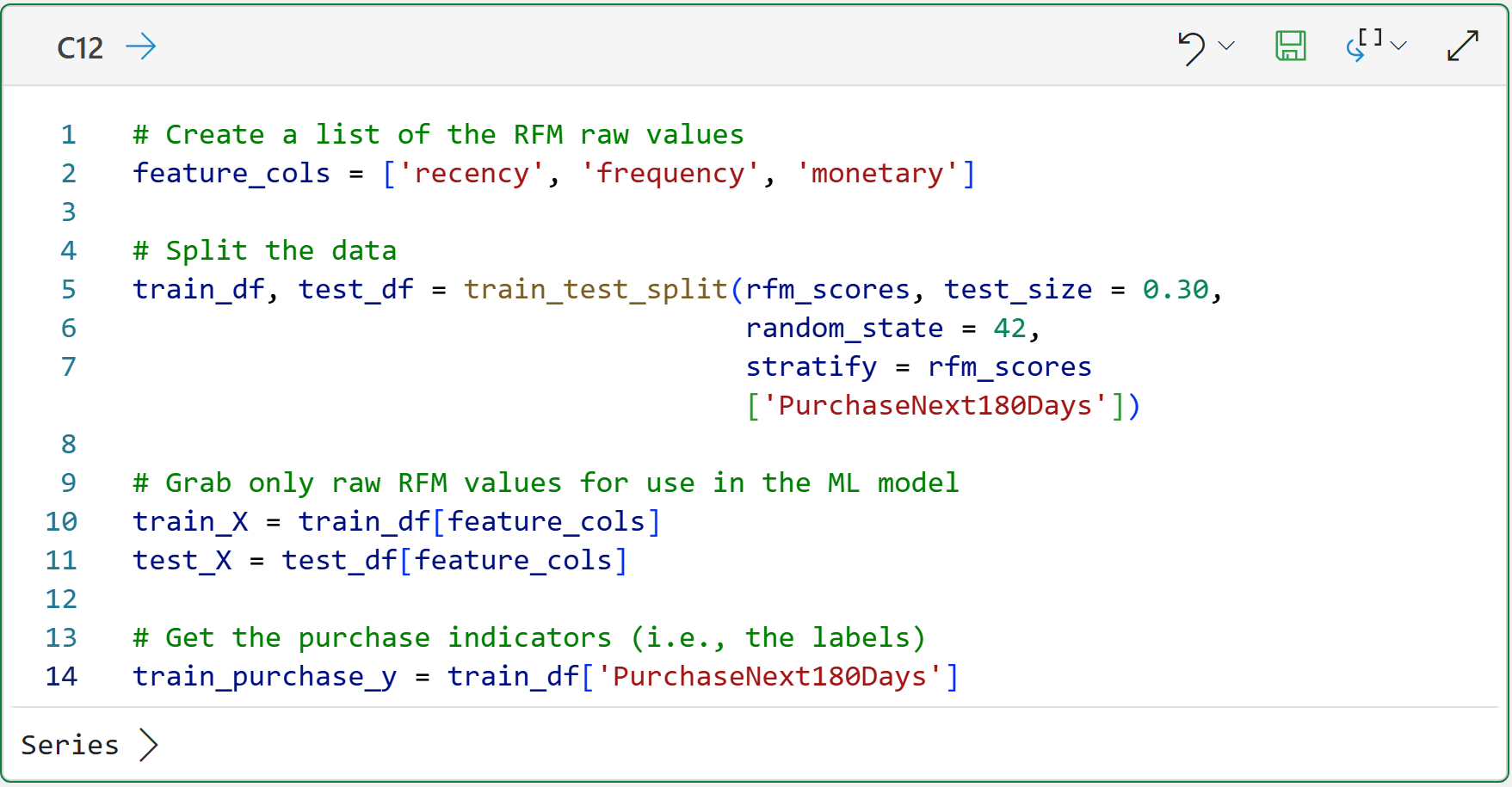
Not surprisingly, the train_test_split() function does all the work:
It randomly selects 30% of the data for the test dataset.
The random_state = 42 helps ensure that you see in your workbook the same results you see in this tutorial.
The stratify = rfm_scores['PurchaseNext180Days'] helps make sure the training and test datasets have a similar mix of customers who did and did not purchase in the next 180 days.
Take a look at the code on lines 10 and 11 of cell C12. The code creates two DataFrames of predictive features (as indicated by _X) that will be used to train and test the ML models, respectively.
Notice, however, that these DataFrames include only the raw RFM feature values, not other features such as Customer ID. This is done to ensure that the model learns properly.
Step 7: Train Stage 1 - Will the Customer Purchase?
The Stage 1 machine learning model will be trained to predict whether a customer is likely to purchase in the next 180 days.
Given that the model is predicting distinct categories (e.g., yes/no, 1/0, true/false, etc.), this is a classification problem, so you will use a RandomForestClassifier:
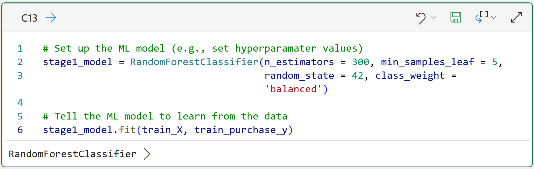
You can think of this model as asking:
Based on the customer's recency, frequency, and monetary values as of June 1, 2011, how likely are they to buy in the next 180 days?
The model does not yet return CLV. It returns the probability that a customer will purchase. For example:
This customer has a 72% chance of purchasing in the next 180 days.
This is the first half of the CLV prediction formula.
Step 8: Train Stage 2 - If They Purchase, How Much Will They Spend?
Stage 2 predicts future revenue, but only for customers who actually purchased in the future window (i.e., for 180 days after June 1, 2011). This is important.
Stage 2 is not trying to learn why some customers have zero revenue. Stage 1 already handles that. Stage 2 is trying to answer:
If this customer buys, how much revenue should we expect?
Here's the code to train a HistGradientBoostingRegressor machine learning model to predict revenue for buyers:
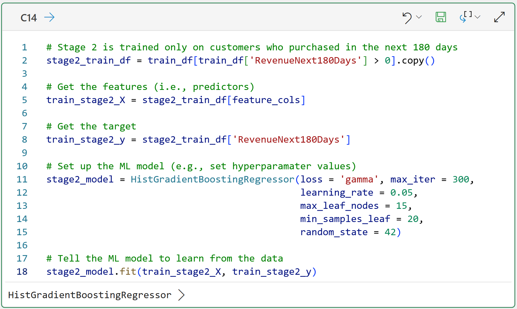
Take a look at the comment on line 10 of cell C14. You can think of ML models as being general-purpose engines that can work with many different kinds of datasets.
Not surprisingly, these engines don't perform optimally right out of the box for any given dataset. Just like automobile engines, ML models need to be tuned for optimal performance.
For example, you will need to tune an ML model differently for a marketing dataset compared to a healthcare dataset.
The hyperparameter values in cells C13 and C14 are used to tune the models. The values provided are unlikely to be the best for the given datasets. I would encourage you to experiment with different hyperparameter values to see if you can improve the predictive performance.
The loss = 'gamma' hyperparameter is useful here because Stage 2 revenue is positive and usually skewed. In plain English, skewed means that a small number of customers spend much more than everyone else.
This is extremely common in CLV analysis. So, don't experiment with this hyperparameter for tuning. Keep it as is.
Step 9: Make CLV Predictions
Now comes the fun part. It's time for you to make and combine the two ML model predictions:
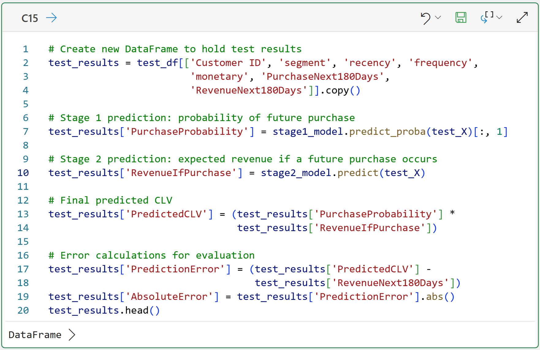
Clicking on the card for cell C15 in the worksheet gives you a preview of test_results:
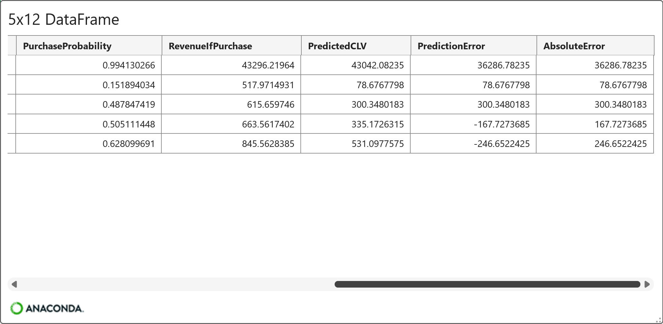
Looking at the preview above, a few things are worthy of note:
PredictiveCLV = PurchaseProbability x RevenueIfPurchase
PredictionError = PredictiveCLV - RevenueNext180Days
AbsoluteError = PredictionError as a positive number (i.e., the absolute value)
Take a close look at the AbsoluteError feature. It demonstrates that predictive CLV is not an exact science, as errors can vary tremendously (e.g., by $36,287).
This is why it's critical to remember that you shouldn't think of your ML models in terms of being correct or incorrect because every ML model will be incorrect to some degree.
Instead, you should think of your ML models as being useful for decision-making despite any errors they might make.
Step 10: Evaluate CLV Predictions
There are many ways to evaluate a predictive model. For this tutorial, you will keep things practical and focus on two metrics: MAE and bias.
MAE stands for mean absolute error. In plain English:
On average, how far away are the predictions from the actual values?
Bias is the average prediction error. In plain English:
Is the model generally predicting too high or too low?
Here's the code to calculate these metrics and store them in a DataFrame:
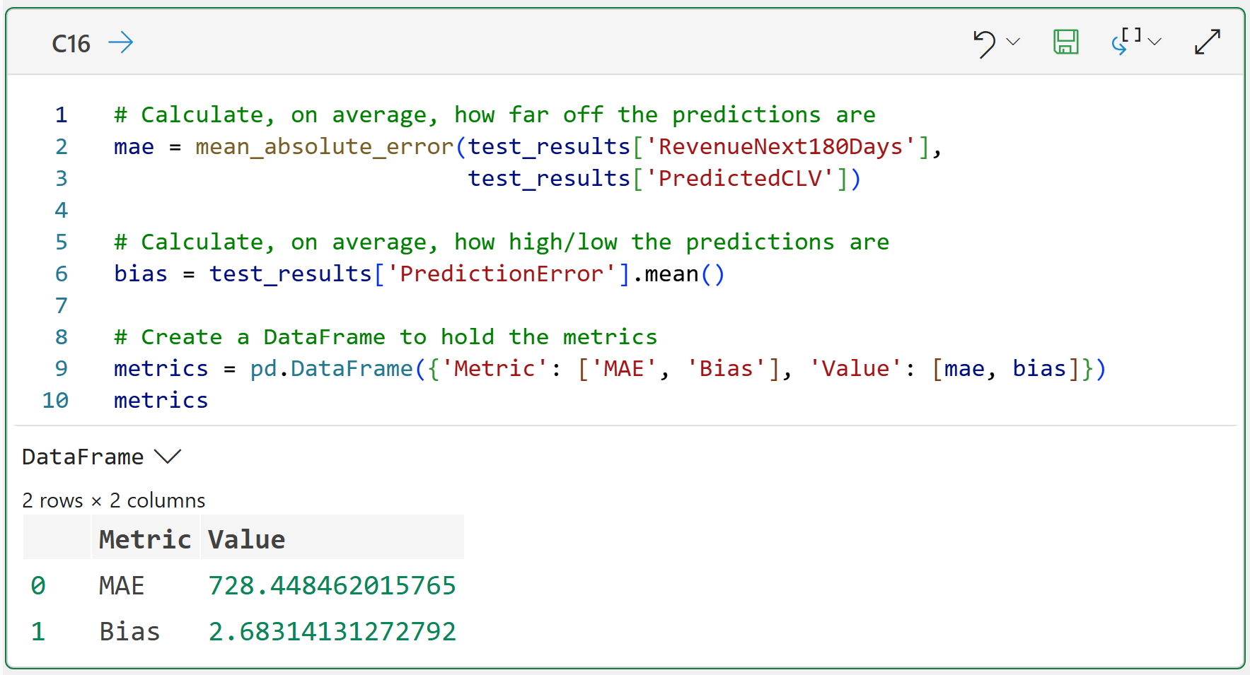
Here's what the metrics are telling you:
On average, the PredictedCLV values are off by $728.45.
On average, the PredictedCLV value is $2.69 too high.
Keep in mind that these metrics are not inherently good or bad without context.
For example, if you are using CLV to make marketing budget decisions, over-predicting can lead to overspending.
If you are using CLV to identify retention opportunities, under-predicting can lead you to overlook customers who are more valuable than they appear.
So, you should always be deliberate in understanding what business levers you're trying to help by predicting CLV.
Also, keep in mind that the calculated metrics are only one way of evaluating the quality of your predictive CLV.
Step 11: Visualize Predicted CLV by Decile
For CLV, ranking customers is often more useful than predicting the exact dollar amount.
Why?
Because many business decisions are prioritization decisions:
Which customers should Sales call first?
Which customers should receive a retention offer?
Which customers should be excluded from expensive campaigns?
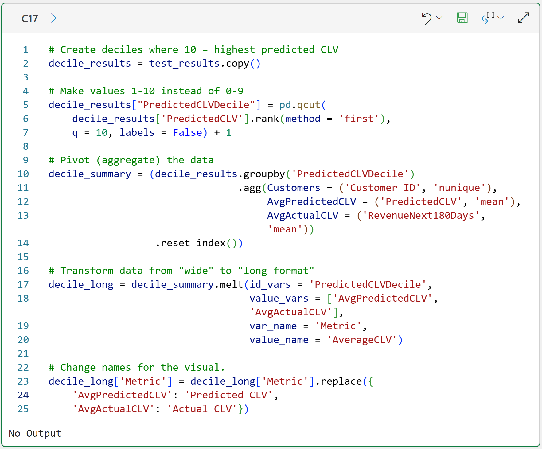
The visualization below groups customers into ten buckets based on predicted CLV. These buckets are called deciles. The following code sets up the deciles for the visualization:
With the data prepared, here's the code to create the visual using plotnine:
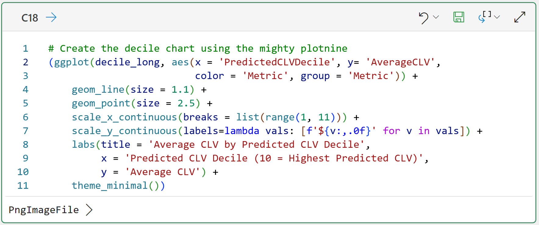
Clicking PngImageFile > displays the visualization:
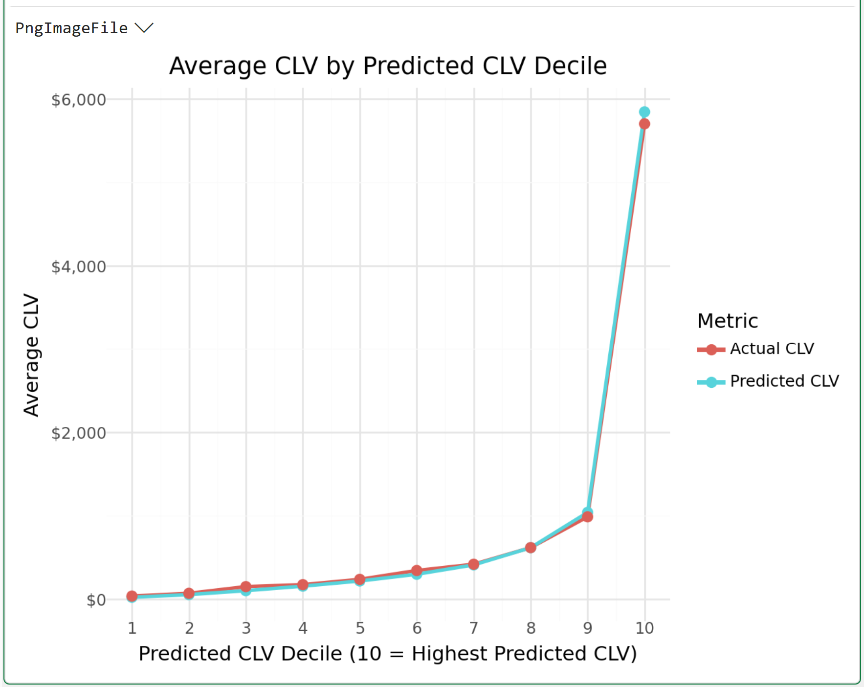
This is one of the most important visuals you can create for your business stakeholders.
If the CLV predictions are to be useful, customers in the higher-predicted-CLV deciles should generally have higher actual future revenue. The relationship does not need to be perfect, but it should be accurate (i.e., the lines should be close).
And that's what we see in this visual.
What You Just Built
Take a step back and look at what happened:
You started with cleaned transaction-level data.
You created RFM features using only purchases before a cutoff date.
You created an 180-day future revenue target using purchases after the cutoff date.
Then you built two models:
A model to predict whether a customer would purchase.
A model to predict how much a customer would spend if they purchased.
Finally, you combined the two predictions:
Predicted CLV = Purchase Probability × Revenue If Purchase
This is a practical predictive CLV model. Not perfect. Not magical.
But much more useful than one average CLV number applied to every customer.
Important Limitations
This tutorial is intentionally beginner-friendly. That means there are limitations. The biggest limitation is that we used a single cutoff date.
For a production CLV project, I would usually create multiple cutoff dates and train the model across many historical prediction windows.
That setup gives the model more examples and better simulates how it would be used in the real world.
You also used a simple customer-level train/test split. That is fine for learning.
But for production, time-based validation is usually safer because it asks the most realistic question:
If we trained the model using the past, how well would it predict the future?
There are other limitations too:
You predicted revenue, not profit.
You used only raw RFM features.
You did not include product mix, country, returns, marketing history, or customer acquisition channel.
You did not tune the model parameters.
You did not calibrate the Stage 1 probabilities.
Those are not failures. They are the next steps.
The goal of this tutorial was to teach the core predictive CLV workflow without burying you in complexity.
That's it for this week.
My next newsletter will continue this tutorial series by teaching you the CAC:LTV ratio and how you use CLV to drive customer acquisition decisions.
Stay healthy and happy data sleuthing!

Dave Langer
Whenever you're ready, here are 3 ways I can help you:
1 - The future of Microsoft Excel is unleashing the power of do-it-yourself (DIY) analytics using Python in Excel. Do you want to be part of the future? My Python in Excel Accelerator online course will teach you what you need to know, and the Virtual Dave AI tutor is included!
2 - Are you new to data analysis? My Visual Analysis with Python online course will teach you the fundamentals you need - fast. No complex math required, and the Virtual Dave AI Tutor is included!
3 - Cluster Analysis with Python: Most of the world's data is unlabeled and can't be used for predictive models. This is where my self-paced online course teaches you how to extract insights from your unlabeled data. The Virtual Dave AI Tutor is included!