
Join 1,000s of professionals who are building real-world skills for better forecasts with Microsoft Excel.
Issue #22 - Machine Learning with Python in Excel Part 2: Profiling Data
This Week’s Tutorial
I'm going to repeat this throughout the tutorial because it's so important:
99% of the Python in Excel code you write is the same as any other Python technology (e.g., Jupyter Notebooks).
What I teach in my free Python Crash Course 100% applies to Python in Excel.
Please read Part 1 of this tutorial series if you haven't already.
If you want to follow along by writing code (highly recommended), you can get the PythonInExcelML.xlsx workbook from the newsletter GitHub repository.
BTW - I've updated PythonInExcelML.xlsx with new data for this tutorial.
OK. Let's get started.
The first five tutorials of this newsletter teach you how to profile your data for building the most useful machine learning models.
These tutorials use one of my favorite Python libraries, ydata-profiling. Unfortunately, Python in Excel doesn't have this library at the time of this writing.
This week's tutorial will teach you Python in Excel alternatives to ydata-profiling. Please note the following:
This tutorial will not cover the "why" of data profiling because I covered that in the first five issues of this newsletter.
You must profile your data before using it to craft a machine learning model. If you don't, you're playing with 🔥.
Compared to ydata-profiling, the Python in Excel experience is more work.
In a future newsletter, we will see if the Copilot in Excel AI can speed things up.
You'll rely heavily on pandas when profiling data using Python in Excel. So, the first step is to load the data into a DataFrame:

Next, the info() method from the DataFrame class provides useful summary information about the dataset:


The Python Editor output above shows that the dataset comprises 15,015 rows (i.e., entries) and 16 columns.
Next, we get a breakdown of each column:
Two things in the above output are critical for crafting useful machine learning models:
The data types (i.e., Dtype) of each column in the dataset.
If there is any missing data.
The info() method output tells us the count of non-null values for each column. This is the count of the data present.
We must compare this count to the dataset's total number of rows to determine if any data is missing. In this case, we know there are 15,016 rows of data.
Looking at each column, we can see that no data is missing (e.g., the HoursPerWeek column has 15,016 non-null values).
Next, we can get summary statistics for each numeric column (or feature) using the describe() method:

Clicking Series in the Python Editor output shows us the results:

A couple of things to note in the Series output above:
The count is non-null values only.
All summary statistics ignore missing (i.e., NaN) values.
The DataFrame class also has a describe() method that does the same across all columns. However, I find this less valuable because the output is much more challenging to read.
Moving on, it's time to check the cardinality of the column using the nunique() method:

The Python Editor output shows 71 unique values in the Age feature.
You also want to check the distribution of your numeric features. My go-to library for data science visualization with Python is the mighty plotnine:

Clicking PngImageFile in the Python Editor output displays the histogram:

If you need help reading and using histograms, check out my Visual Analysis with Python online course.
As you are profiling your numeric features, you should always be asking yourself this question:
"Does what I'm seeing make sense given the business nature of the data?"
Whenever the answer is "No," you must dive into the data and discover why. This often includes speaking to business subject matter experts.
The last thing to check is whether your numeric features are monotonic. Here's a simple utility function you can use:

Remember - If a numeric feature is monotonic, never use it in a machine learning model unless you know for sure it isn't going to be a problem
Most monotonic numeric features are forms of unique identifiers, and these should never be used in machine learning models!
For more details on how to profile numeric features, check out newsletter issue #2.
It's time to move on to categorical features:

The output above provides the following information about the Occupation categorical feature:
The count of non-null values (i.e., 15,016).
The cardinality (i.e., count) of the feature's unique values (i.e., levels).
The most frequently occurring level value (i.e., Exec-managerial).
The frequency of this level value (i.e., 2,621 out of 15,016).
Next, you want to look at the frequencies of the level values:
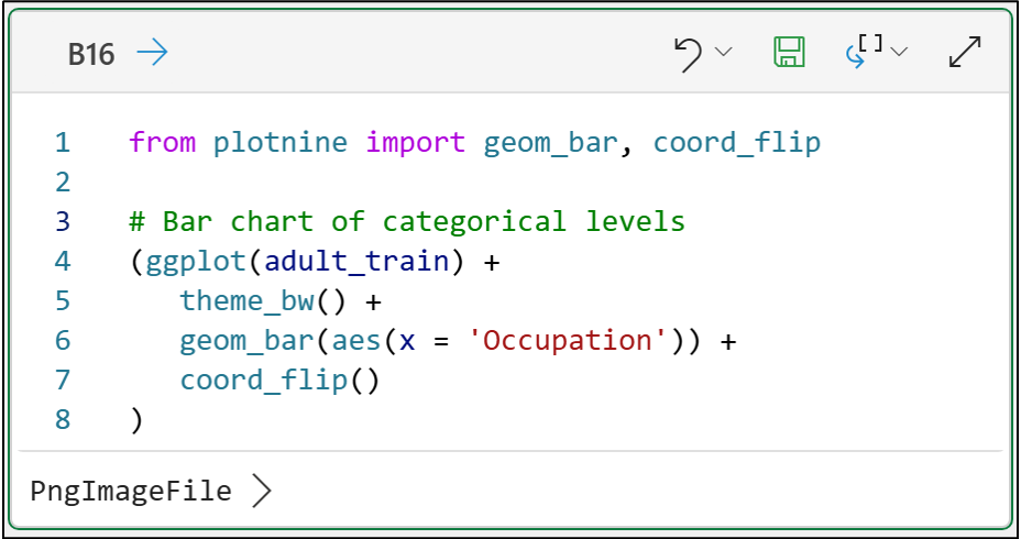

Horizontal bar charts (using coord_flip() in the code above) are one of the best ways to investigate the frequency of categorical levels.
For more details on how to profile categorical features, check out newsletter issue #3.
Date-time data is very common in business analytics. More importantly, some of the most powerful features for your machine learning models can be engineered from date-time data.
However, date-time data is particularly problematic because often the data is dirty. This makes profiling it a must:

In the output above, we can see the following about the CollectionDate feature:
There are 15,016 non-null values.
The minimum date is 1994-01-03.
The maximum date is 1994-12-30.
You will also want to check the frequency of the date-time values using a bar chart:


The bar chart of the CollectionDate feature shows that, overall, the frequency of individual date-time values are quite similar.
Once again, this aligns with our fundamental data profiling question:
"Does what I'm seeing make sense given the business nature of the data?"
For more details on how to profile date-time features, check out newsletter issue #4.
I'll need to save profiling text data for another tutorial series because text data requires a lot of preprocessing.
I'll conclude this tutorial with profiling correlation and duplicate data. To learn about the "why" of this profiling, check out newsletter issue #5.
Getting the correlation between numeric features is easy using the corr() method of the DataFrame class:
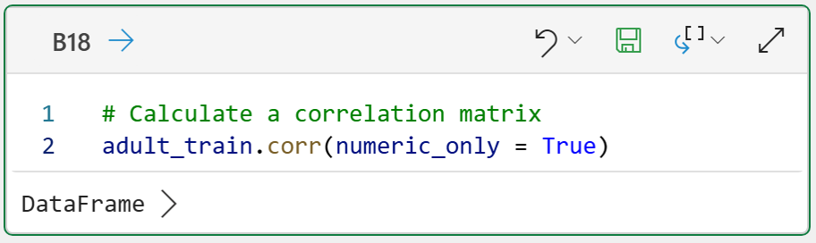
Unfortunately, viewing the DataFrame returned by the corr() method in the Python Editor output doesn't work because of its size.
Luckily, you can have the DataFrame spilled to the worksheet by changing the output of the Python formula to Excel value:


The easiest way to assess the correlation between a categorical column and a numeric column is to use a box plot:


The above box plot reveals interesting associations. For example, the Occupation level Exec-managerial has the highest median Age.
If you need help reading and using box plots, check out my Visual Analysis with Python online course.
For assessing the correlation between two categorical columns, a bar chart is a powerful tool:


In the bar chart above, you're looking for bars where one color (i.e. level) is dominant. For example:
The Priv-house-serv level is completely green (i.e., Private).
The Armed-Forces level is completely reddish-orange (i.e., Federal-gov).
The following code will output any duplicate rows to the worksheet for you to inspect:


NOTE - The above code removes the CollectionDate feature to demonstrate duplicate rows. Without removing CollectionDate, there are no duplicate rows.
Whew!
That was a long tutorial, but I hope I'm proving to you what a game-changer Python in Excel is for professionals wanting to make an impact at work with DIY data science.
This Week’s Book
DIY data science with Microsoft Excel is nothing new. This week's book recommendation was first published all they way back in 2010!
This book was an eye-opener for me as to what actually is possible with Microsoft Excel. For example, implementing logistic regression predictive models using the Solver:

If you're unable to get access to Python in Excel for whatever reason (e.g., your IT department blocks access), this book uses accessible Excel features like the Solver.
However, as much as I love this book, it is obsolete now that we have Python in Excel.
That's it for this week.
Next week's newsletter will demonstrate using Python in Excel to conduct a customer segmentation.
Stay healthy and happy data sleuthing!

Dave Langer
Whenever you're ready, here are 3 ways I can help you:
1 - The future of Microsoft Excel forecasting is unleashing the power of machine learning using Python in Excel. Do you want to be part of the future? Order my book on Amazon.
2 - Are you new to data analysis? My Visual Analysis with Python online course will teach you the fundamentals you need - fast. No complex math required, and Copilot in Excel AI prompts are included!
3 - Cluster Analysis with Python: Most of the world's data is unlabeled and can't be used for predictive models. This is where my self-paced online course teaches you how to extract insights from your unlabeled data. Copilot in Excel AI prompts are included!