
Join 1,000s of professionals who are building real-world skills for better forecasts with Microsoft Excel.
Issue #30 - Market Basket Analysis Part 5:
Feature Engineering
This Week’s Tutorial
This week's tutorial focuses on engineering features for market basket analysis (MBA).
If you're new to the newsletter and need to catch up, check out Parts 1-4 of this tutorial series via the newsletter back issues.
When professionals first learn MBA, a common reaction is something like this:
"Wait a minute, Dave. You mean I can only use binary features with MBA? That seems like a huge problem for my analysis/domain/business problem!"
As it turns out, the requirement for using binary features is actually quite common in DIY data science. Here are two examples:
Linear/Logistic regression requires transforming categorical data into binary features.
Many machine learning algorithms offered by Python's scikit-learn library require transforming categorical data into binary features.
So, don't underestimate the power of MBA simply because you need to use binary features!
As you build your DIY data science skills, a common theme across the techniques you use will be spending more time working with the data (i.e., writing code) than you do writing code to perform the actually analysis.
Many years ago, research was conducted on data mining projects (think of the term data mining as what data science was called back then). The research showed that between 60-80% of project effort was devoted to tasks like:
Getting access to the data.
Understanding the data.
Cleaning the data.
Based on my experience as an analytics consultant, nothing has changed in 2025.
These days, it's common to refer to all of these data-related activities as data wrangling.
While all of these activities are critical for success, one aspect of data wrangling is the most important: feature engineering.
In this regard, successful use of MBA is no different than logistic regression or random forest predictive models.
The best results come from the best features.
In this tutorial, you are going to learn the following two patterns that I've used with MBA to provide insights that have delighted business stakeholders:
Presence
Magnitude
Let's dive in.
Presence Features
This MBA feature pattern is what you're already familiar with from the tutorials in this series.
Using the grocery store example from previous tutorials, whether or not a purchase (i.e., a transaction) contains whole milk.
The following DataFrame illustrates a hypothetical grocery store dataset build around presence features:

While the above dataset uses ones and zeros to indicate presence, the values of True/False could be used instead, as Python treats them as equivalent.
If you've been a long-time subscriber to this newsletter, you will recognize the above dataset as being very similar to one-hot encoding.
One-hot encoding is a common technique for transforming categorical features into a binary representation (e.g., for use with the scikit-learn library).
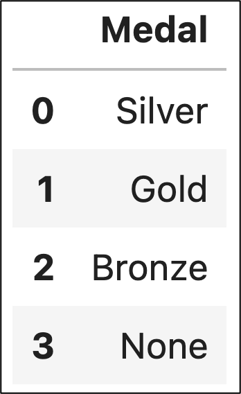
Imagine you have a dataset tracking the results of the Olympic games with a Medal feature to track each athlete's results like the following:
After one-hot encoding the Medal feature, the resulting DataFrame would look something like this:
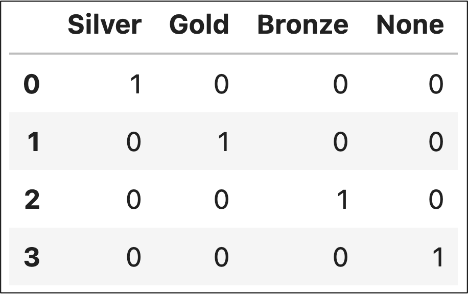
The result of one-hot encoding is a presence indicator (e.g., 1/0) and can be used with MBA.
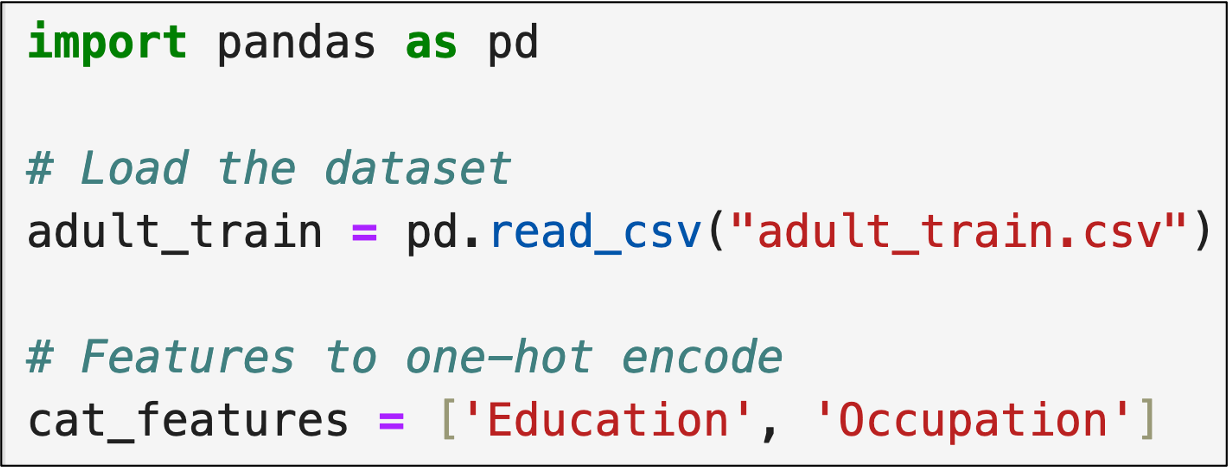
The following code demonstrates how to use one-hot encoding with categorical columns from the adult_train.csv dataset available from the newsletter's GitHub repository.
First up, loading the data using Jupyter Notebook:
And using Python in Excel:

Python's scikit-learn library offers the OneHotEncoder class to do exactly what we need to transform categorical data for MBA:


In the code samples above, please note the following:
As usual, the Python code is the same regardless if you use Jupyter Notebook or Python in Excel.
The OneHotEncoder object is coded to output a DataFrame - this is usually what you want.
The OneHotEncoder object is only encoding the two features specified by cat_features.
The one-hot encoded data is returned and stored as train_cat.
And here's the output from the above code:
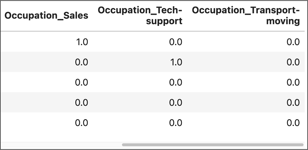
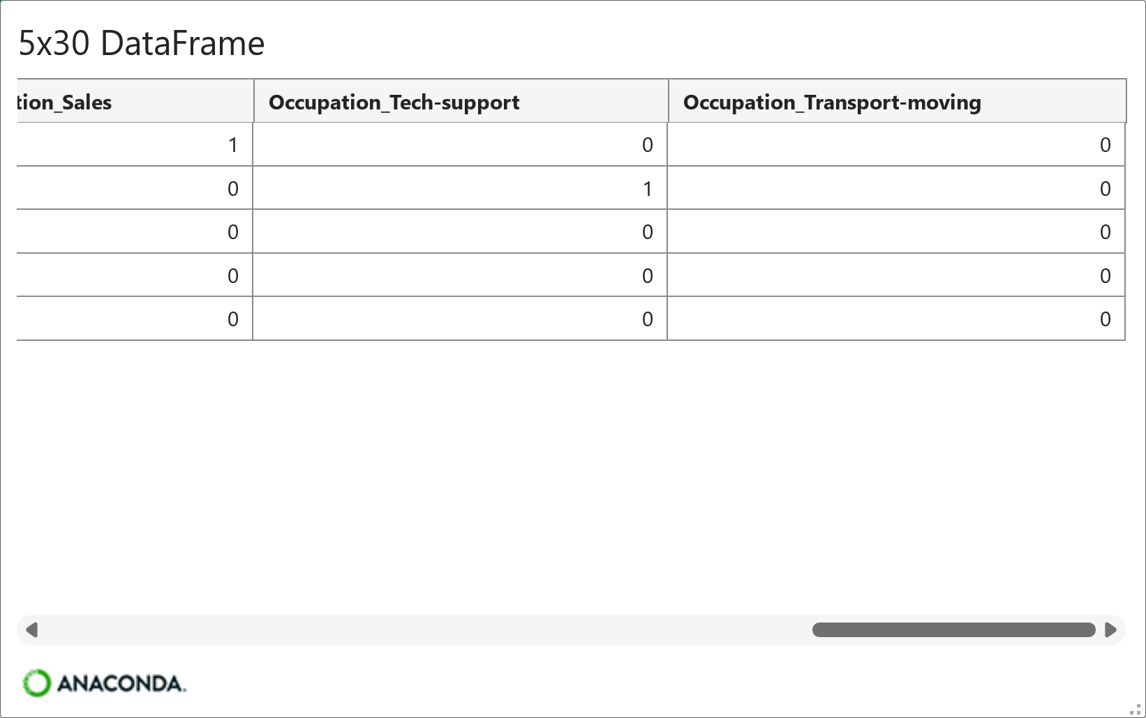
As shown in the above outputs (i.e., Jupyter Notebook and Python in Excel, respectively), the horizontal scroll bar shows that there are many more one-hot encoded columns to the left not depicted in the images.
Also note the Occuptation_ prefix for each feature name. This is a naming convention that tells you which original feature was the source of the one-hot encoding (i.e., the Occupation feature).
But that's not all.
There are many instances where you have a numeric feature that can easily be wrangled into presence features for MBA.
The running grocery store example of this tutorial series is a prime example. Regardless of the count of a particular product within a transaction (e.g., three bottles of mustard), a simple binary indicator is all that is needed.
There are also times where numeric features do not represent counts, but a simple binary indicator of non-zero status is more than sufficient for MBA.
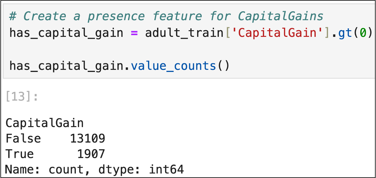
A great example of this situation is the CapitalGain feature of the adult_train.csv dataset. Since the distribution of this feature is highly skewed (i.e., most values are 0), a simple presence feature is highly useful for MBA.
The following Jupyter Notebook code demonstrates how to perform this transformation. Since the code is the same for Python in Excel, I will not show Excel for brevity:
As you might imagine, the two examples covered here are not the only way you can create presence features. The possibilities are endless. Here are two more to spark your creativity:
Detecting the presence of a substring in text data.
Detecting if a behavior occurred within X amount of time.
However, I've found that I've used the two techniques covered in this section more often than any others when creating my presence features for MBA.
Magnitude Features
Your MBA can often be more effective if the magnitudes of numeric features can be included as binary indicators. Making this happen is the result of a two-step process:
Transforming the values of numeric features into categories.
One-hot encoding the categories.
The first step is more common than you might imagine in analytics and is often referred to as binning. Here are some examples:
Creating histograms requires defining bins for numeric feature data.
Decision tree-based machine learning algorithms bin numeric features as part of their learning process.
Using deciles to bin numeric feature data for RFM analysis.
I'll use the last example of RFM analysis to demonstrate a useful technique for creating magnitude features for MBA. First up, RFM stands for:
(R)eceny
(F)requency
(M)onetary
RFM analysis is an old-school marketing analysis technique where you classify customers based on their RFM score.
The most common (but not only) way to calculate the RFM score is by applying the following logic to each of the three RFM features:
Classify each value of each feature in terms of deciles (i.e., bin the values into 10 distinct groups).
The top 10% of values receive a score of 9.
The next top 10% of values receive a score of 8.
And so on, until the bottom 10% of values receive a score of 0.
To cement this type of feature engineering, I will demonstrate using the HoursPerWeek feature from the adult_train.csv dataset.
The HoursPerWeek feature embodies a common problem when using deciles with business data - there are often a lot of duplicates.
For example, based on the business nature of the feature, many of the HoursPerWeek values are 40 (i.e., the standard US work week).
When there are many duplicate values, it can make creating deciles impossible.
So, the following code demonstrates using the rank() method first to transform the data such that it can be cleanly binned into deciles.
The code tells rank() to assign a value based on position. For example:
The first value of 40 found would be assigned a rank of 1.
The second value of 40 found would be assigned a rank of 2.
And so on.
The code then calls the qcut() method from pandas to divide the rankings into deciles (i.e. q = 10). The following shows the code and the results:
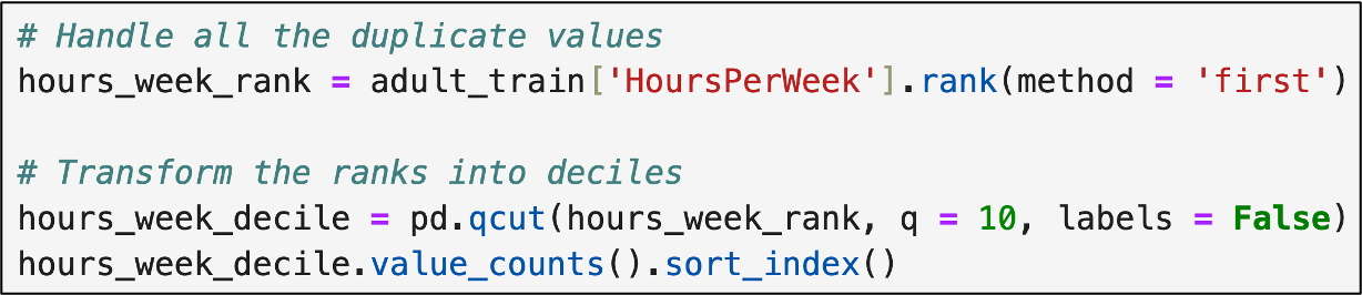

Note - The code is the same whether you're using Jupyter Notebook or Python in Excel.
With the HoursPerWeek feature transformed into categorical magnitudes, the next step is to use a OneHotEncoder to transform the data.
The following code calls the to_frame() method because the OneHotEncoder expects a DataFrame object:


Voila! Magnitudes transformed to a format to include in your MBA.
As with presence features, there are many possibilities for engineering magnitude features for MBA. Once again, however, I've found that using the combination of rank() and qcut() is what I've overwhelming used in my analyses.
I hope this tutorial has gotten you excited about the possibilities of using MBA in your own work. As I mentioned in a previous tutorial, I've found over the years that insights born of MBA resonate with business stakeholders.
This Week’s Book
Since MBA is often used to analyze customer behaviors, the following book is a useful to anyone getting started in the space:
Two things that are super important to note. First, MBA can be used to analyze just about anything, not just customer behaviors. Second, the lessons in this book are applicable to many areas beyond customer analytics.
That's it for this week.
Next week's newsletter will conclude the tutorial series by covering Copilot in Excel AI prompts for performing MBA - including feature engineering.
Stay healthy and happy data sleuthing!

Dave Langer
Whenever you're ready, here are 3 ways I can help you:
1 - The future of Microsoft Excel forecasting is unleashing the power of machine learning using Python in Excel. Do you want to be part of the future? Order my book on Amazon.
2 - Are you new to data analysis? My Visual Analysis with Python online course will teach you the fundamentals you need - fast. No complex math required, and Copilot in Excel AI prompts are included!
3 - Cluster Analysis with Python: Most of the world's data is unlabeled and can't be used for predictive models. This is where my self-paced online course teaches you how to extract insights from your unlabeled data. Copilot in Excel AI prompts are included!